How to Train Your Intercept

using AlgebraOfGraphics
using CairoMakie
using Random
using ProjectRoot
using LaTeXStrings
using JLD2
using GLM
using LinearAlgebra
using DataFrames
using CSV
using Statistics
import QuartoNotebookWorker

output_format = QuartoNotebookWorker.notebook_options()["format"]["pandoc"]["to"]
is_pdf = output_format in ("pdf", "latex")

function output_size(size)
    width, height = size
    # scale = min(500 / 800, 500 / width)
    scale = 0.75
    return is_pdf ? round.(Int, scale .* size) : size
end

set_theme!(theme_latexfonts(); fontsize = is_pdf ? 12 : 14, size = output_size((800, 450)))

Random.seed!(14)

strategy_labels = Dict(
    :bt_gradient => "Armijo gradient",
    :exact => "Exact",
    :gradient => "Gradient",
    :newton => "Newton",
    :unguarded_newton => "Bare Newton",
)
strategy_label(strategy) = get(strategy_labels, Symbol(strategy), string(strategy))

# A run that terminates early must retain its converged state in passwise
# summaries; otherwise the seed cohort changes as runs finish.
function carry_forward(values, length_out)
    isempty(values) && throw(ArgumentError("cannot carry forward an empty trajectory"))
    length(values) <= length_out ||
        throw(ArgumentError("output length is shorter than input"))
    return vcat(values, fill(last(values), length_out - length(values)))
end

1 Introduction

Popular solvers for regularized generalized linear models (GLMs) agree on coordinate descent (CD) but disagree about one coordinate: the intercept. GLMs usually include this coordinate to represent the baseline response and to absorb constant shifts in the predictors without changing the fitted slopes. It is unpenalized and never drops out of the fitted model, yet solvers update it in different ways. Research on coordinate descent has examined acceleration, parallelization, and convergence rates, but has largely treated the intercept update as a routine implementation choice. That choice can dominate convergence speed when the response is imbalanced. For direct coordinate descent, a single safeguarded Newton step per pass removes this slowdown in our experiments.

The disagreement follows a deeper split among implementations. Some solvers, including skglm¹ (Bertrand et al. 2022), run coordinate descent directly on the original GLM loss. Others repeatedly replace that loss with a quadratic approximation and solve the approximation by coordinate descent. A local quadratic already contains the current intercept curvature, so the update strategies coincide within it. A quadratic built from a worst-case curvature bound retains the same problem as the conservative direct update. The six production solvers in Section 4.6 use these designs. We explain in Section 3 and Section 3.4 when the distinction matters.

We study the optimization problem \[ \mathop{\mathrm{minimize}}_{\beta_0 \in \mathbb{R},\beta \in \mathbb{R}^p} \Big( P(\beta_0,\beta) = F(\beta_0, \beta) + G_{\lambda}(\beta) \Big) \tag{1}\] where \(P\) is the primal objective, \(F\) is the loss, and \(G_\lambda\) penalizes large coefficients while leaving the intercept unpenalized. Throughout the paper, we assume that \(G_\lambda\) is a proper, closed, convex, separable penalty and that \(F\) is the loss averaged over observations, \[ F(\beta_0, \beta) = \frac{1}{n}\sum_{i=1}^n f(x_i^\top \beta + \beta_0; y_i), \] where \(f\) is smooth, twice differentiable, and convex. Averaging by \(n\) keeps the global Lipschitz constant for the intercept, \(L_0 = \sup f''\), independent of \(n\). It also matches the objective scaling of the production solvers that we compare in Section 4.6: \((1/n) \cdot \text{loss} + \lambda \|\beta\|_1\). For brevity, we write \(x_i\) for the \(i\)th row of the design matrix \(X\) and \(x_j\) for its \(j\)th column, and we let \((\hat{\beta}_0, \hat{\beta})\) denote a solution to Equation 1. Under these assumptions, \(P\) is a convex composite objective. The assumptions cover every penalty and model in our analysis and experiments. We do not consider nonconvex penalties.

We compare three strategies for updating the intercept once per pass over the coefficient coordinates:

Gradient Strategy

Takes a single gradient step based on a global curvature bound.

Newton Strategy

Takes a single Newton step based on the curvature at the current iterate, with an Armijo backtracking line search to guard against overshooting.

Exact Strategy

Minimizes the loss over the intercept while holding the coefficients fixed.

In the analysis, exact means setting the intercept to its conditional minimizer. The experiments compute this minimizer numerically, with tolerances documented in Supplement S3.

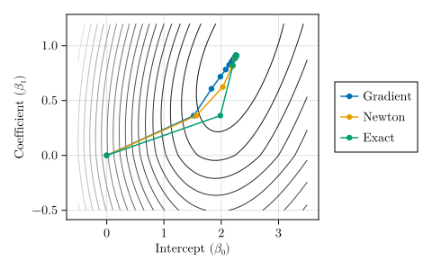
These strategies can converge at substantially different rates when the response is imbalanced—for example, when positive cases are rare in logistic regression. The three paths in Figure 1 trace the strategies across the level sets of Equation 1 for a toy problem with one feature and an intercept. The gradient strategy approaches the solution through many small steps, whereas the Newton and exact strategies reach it in only a few.

Random.seed!(42)

n = 100
p = 1
k = 10
μ0 = 0.9

X, y = generatedata(
    n,
    p;
    response = :binomial,
    μ0 = μ0,
    x_type = :normal,
    x_density = 0.9,
    ρ = 0.99,
    s = k,
    amplitude = 1,
)

strategies = [
    (strategy = GradientStrategy(), name = "Gradient"),
    (strategy = NewtonStrategy(), name = "Newton"),
    (strategy = ExactStrategy(), name = "Exact"),
]

reg = 0.2

results = [
    cdsolver(
        X,
        y,
        reg,
        lossfun = LogisticLoss(),
        intercept_strategy = s.strategy,
        save_history = true,
    )
    for s in strategies
]

λ = results[1].λ

# The solver penalizes standardized coefficients but returns original-scale slopes.
feature_scale = std(X[:, 1]; corrected = false)

β0 = range(-0.5, 3.5, length = 100)
β = range(-0.5, 1.2, length = 100)
grid = [(b0, b) for b0 in β0, b in β]

primal_values = zeros(size(grid))

for (i, (b0, b)) in enumerate(grid)
    η = b0 .+ X[:, 1] * b
    primal_values[i] = loss(LogisticLoss(), η, y) + λ * feature_scale * abs(b)
end

fig = Figure(; size = output_size((480, 300)))
ax = Axis(fig[1, 1], xlabel = L"Intercept ($\beta_0$)", ylabel = L"Coefficient ($\beta_1$)")

levels = geomspace(minimum(primal_values), maximum(primal_values), 20)

contour!(β0, β, primal_values, levels = levels, colormap = :grays)

for (res, s) in zip(results, strategies)
    scatterlines!(res.intercepts, dropdims(res.coefs, dims = 1), label = s.name)
end

fig[1, 2] = Legend(fig, ax)

fig

Figure 1: Intercept-update trajectories on a toy logistic problem. The paths show the iterates of the gradient, Newton, and exact strategies over the objective level sets for a one-feature model with an intercept.

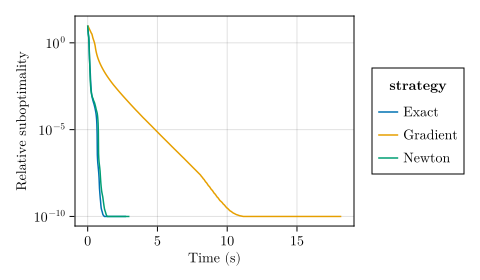
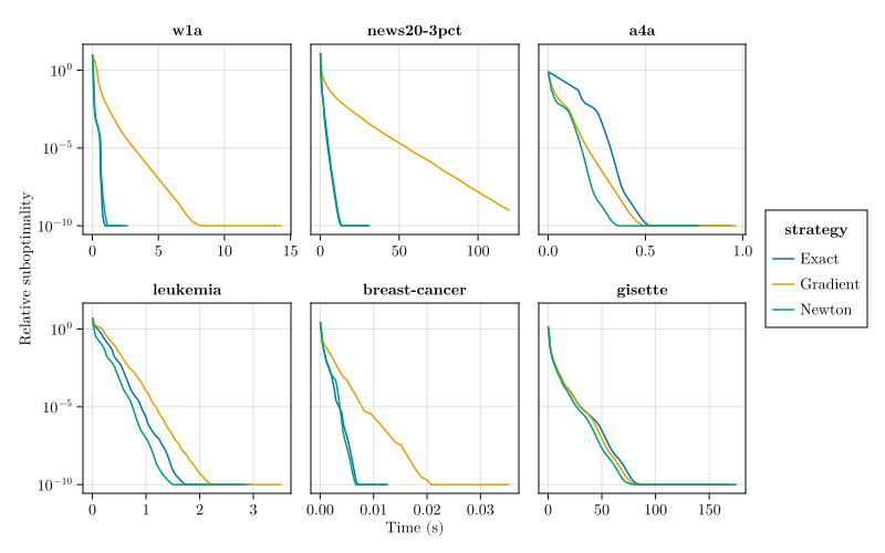
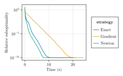
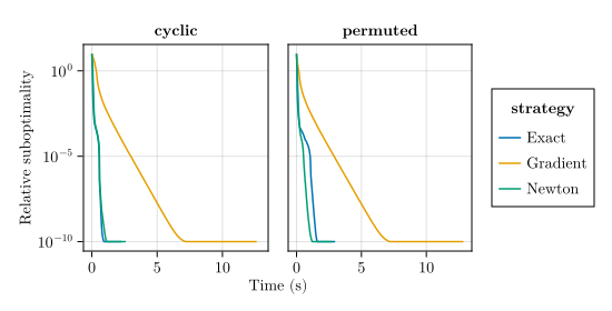
In Figure 2, we compare how quickly the three strategies converge when fitting \(\ell_1\)-regularized logistic regression to the w1a dataset (Platt 1998). The Newton and exact strategies bring the relative suboptimality bound below \(10^{-8}\) after roughly 45 passes, while the gradient strategy takes more than seven times as many.

dd = JLD2.load(@projectroot("results", "first-example.jld2"))
df = DataFrame(dd["results"])
df = flatten(df, [:time, :relgaps, :gaps, :primals])

df.relgaps .= max.(df.relgaps, 1.0e-10)
df.strategy = strategy_label.(df.strategy)

spec = data(df) * mapping(:time, :relgaps, color = :strategy)

layers = visual(Lines)

draw(
    layers * spec,
    axis = (; yscale = log10, ylabel = "Relative suboptimality", xlabel = "Time (s)"),
    figure = (; size = output_size((480, 280))),
)

Figure 2: Overall convergence on w1a. The plot shows a relative suboptimality bound versus time for the three intercept strategies in \(\ell_1\)-regularized logistic regression.

We make four contributions:

• We formalize three strategies for updating an unpenalized intercept: gradient, Newton, and exact minimization.

• We use a Schur complement to describe how an intercept update changes the coefficient gradients. A frozen quadratic model then explains why, under strong coupling, the gradient-to-Newton pass-count ratio approaches the ratio of global to local intercept curvature.

• We classify CD-based GLM solvers by their treatment of curvature and the intercept, and we evaluate six production solvers using controlled comparisons where possible.

• We extend the analysis to multinomial logistic regression, where rare classes create low-curvature directions. Experiments on synthetic and real data show that Newton updates closely match exact minimization and can be much faster than gradient updates.

2 Related work

The choice of intercept update touches three strands of the literature, none of which has analyzed it as a separate problem. The first concerns how CD-based GLM solvers incorporate the intercept. Existing work generally treats this as a routine implementation choice. The glmnet literature (Friedman et al. 2010; Tay et al. 2023), for example, describes two schemes for weighting the inner logistic solver in iteratively reweighted least squares (IRLS): local weights and a global 1/4 upper bound. The software exposes them through type.logistic = "Newton" and "modified.Newton", which the documentation presents as a speed trade-off rather than as a choice of intercept strategy.

LIBLINEAR’s newGLMNET solver (Fan et al. 2008; Yuan et al. 2012) treats the intercept as the unregularized last coordinate of each prox-Newton subproblem. Coordinate descent then optimizes the intercept along with the coefficients. By the end of the inner solve, the intercept has reached its conditional minimum for the quadratic. The solver has no separate intercept loop on the original loss.²

BlitzL1 (Johnson and Guestrin 2015) does the same inside the prox-Newton inner CD solve. After each subproblem, it also runs a capped one-dimensional Newton loop on the original loss to bring the intercept gradient within tolerance.³ celer (Massias et al. 2020) does not support intercepts for \(\ell_1\)-logistic regression. Implementations therefore make varied choices, but previous work has not directly analyzed the response distributions for which those choices matter.

A second thread is the Frisch–Waugh–Lovell tradition of partialling out. In linear regression, the intercept can be handled separately: centering the features decouples it from the slopes and, when the intercept is left unpenalized, gives \(\hat\beta_0 = \bar y\) (Lovell 1963). glmnet leaves the intercept unpenalized on translation-invariance grounds—penalizing \(\beta_0\) would make the path depend on the arbitrary location of \(y\)—and this decoupling makes that choice essentially free under Gaussian loss. After solving for the slopes, the intercept is recovered as \(\hat\beta_0 = \bar y - \bar x^\top \hat\beta\).

For non-Gaussian GLMs, the decoupling fails because curvature varies across observations. Ordinary feature centering no longer removes the interaction between the intercept and the slopes, and the closed form for \(\hat\beta_0\) disappears. adelie (Yang and Hastie 2024) handles this dependence through its proximal quasi-Newton approximation. At each linearization, it builds a weighted Gaussian surrogate and absorbs the intercept into that surrogate rather than treating it as a separate CD coordinate.⁴ For Gaussian data, the framework in Section 3 reduces to the familiar result: the loss has constant curvature, so the gradient and Newton strategies coincide on the intercept.

The third thread is majorization–minimization (MM). The binary logistic curvature bound \(L_0 = 1/4\) is the binary specialization of the quadratic Hessian majorant used by Böhning (1992) to build an MM algorithm for multinomial logistic regression. Hunter and Lange (2004) give the canonical exposition of MM. Krishnapuram et al. (2005) apply Böhning’s bound to L1-penalized multinomial logistic regression, a direct precedent for our multinomial extension.

In regularized logistic regression, the same construction appears in the modified.Newton mode of glmnet and the MM mode of biglasso (Zeng and Breheny 2021) (Table 3). Because the global majorant does not adapt to local curvature, it can produce a much smaller intercept correction than a Newton step when the response is imbalanced. In multinomial regression, the same mismatch appears along directions associated with rare classes. The MM literature treats this as loose majorization. We quantify the resulting slowdown for imbalanced binary and rare-class multinomial problems (Section 3.4, Figure 22).

3 Theory

The three strategies differ in how they respond to intercept curvature. The gradient strategy uses a global upper bound, Newton uses the curvature at the current iterate, and the exact strategy minimizes the intercept subproblem. On imbalanced data, the local curvature can be much smaller than the global bound. When the intercept—or a direction coupling it with a coefficient—controls convergence, this mismatch can make the gradient strategy slower by a factor proportional to the ratio of global to local curvature. We first analyze the effect of one intercept update, then follow its effect through repeated passes on a fixed quadratic model and compare the resulting local rates with experiments.

Throughout this section, we work with the canonical-link GLM loss averaged over observations, \[ F(\beta_0, \beta) = \frac{1}{n}\sum_{i=1}^n f(x_i^\top \beta + \beta_0; y_i). \] We first derive the scalar-intercept results for the Gaussian, binomial, and Poisson models. We later extend them to multinomial logistic regression, whose intercept is a vector. For observation \(i\), let \(\eta_i = x_i^\top \beta + \beta_0\) denote the linear predictor, and let \(g^{-1}\) denote the inverse link. The conditional mean is then \(\mathop{\mathrm{E{}}}(y_i \mid \eta_i) = g^{-1}(\eta_i)\). For the canonical-link models considered here, the derivative of the negative log-likelihood simplifies to the generalized residual, \[ f'(\eta_i; y_i) = g^{-1}(\eta_i) - y_i = r_i. \] All gradients below follow from this canonical-link identity, and all Hessians follow from its derivative. The identity does not hold for arbitrary noncanonical links. The loss, link, and inverse link for the four models we study—Gaussian, binomial, Poisson, and multinomial—appear in Table 1.

Table 1: Loss, link, and inverse-link functions for the GLM families studied. The multinomial row uses the reference-class parameterization with class \(m\) as the reference (\(\eta_m = 0\), \(\mu_m = 1 - \sum_{j<m}\mu_j\)), so \(\eta\) and \(\mu\) in that row are \((m-1)\)-vectors, and \(\log\) and \(\exp\) are applied elementwise.

Model	\(f(\eta; y)\)	\(g(\mu)\)	\(g^{-1}(\eta)\)
Gaussian	\(\frac{1}{2}(y - \eta)^2\)	\(\mu\)	\(\eta\)
Binomial	\(\log(1 + e^\eta) - \eta y\)	\(\log\left( \frac{\mu}{1 - \mu} \right)\)	\(\frac{e^\eta}{1 + e^\eta}\)
Poisson	\(e^\eta - \eta y\)	\(\log(\mu)\)	\(e^\eta\)
Multinomial	\(\log\left( 1 + \sum_{j=1}^{m-1} e^{\eta_j} \right) - \sum_{k=1}^{m-1} y_k \eta_k\)	\(\log\left( \frac{\mu}{1 - \sum_{j=1}^{m-1} \mu_j} \right)\)	\(\frac{\exp(\eta)}{1 + \sum_{j=1}^{m-1} e^{\eta_j}}\)

3.1 Coordinate descent

Coordinate descent updates one coordinate at a time while holding the others fixed. For coefficient \(\beta_j\), the chain rule gives \[ \frac{\partial}{\partial \beta_j} F(\beta_0, \beta) = \frac{1}{n}\sum_{i=1}^n x_{ij} f'(\eta_i; y_i). \]

The smooth part of a coefficient or intercept update takes a step in the negative partial-gradient direction, \[ \beta_j^+ = \beta_j - \gamma_j \frac{\partial}{\partial \beta_j} F(\beta_0, \beta), \] where \(\gamma_j\) is the step size. The usual CD choice is a Newton step, based on the second derivative \[ H_{jj} = \frac{\partial^2}{\partial \beta_j^2} F(\beta_0, \beta) = \frac{1}{n}\sum_{i=1}^n x_{ij}^2 f''(\eta_i; y_i). \]

Letting \(w_i = f''(\eta_i; y_i)\) be the weights, we can rewrite the Hessian diagonal as \[ H_{jj} = \frac{1}{n}\sum_{i=1}^n x_{ij}^2 w_i. \]

This yields the step size \[ \gamma_j = H_{jj}^{-1} = \left( \frac{1}{n}\sum_{i=1}^n x_{ij}^2 w_i \right)^{-1}. \]

For the intercept, the local curvature is \[ H_{00} = \frac{\partial^2}{\partial \beta_0^2} F(\beta_0, \beta) = \frac{1}{n}\sum_{i=1}^n f''(\eta_i; y_i). \] The corresponding Newton step size is \(\gamma_0 = H_{00}^{-1}\). Production solvers, however, use three different intercept updates:

1. A Newton step, setting \(\gamma_0\) as above.
2. A gradient descent step, setting \(\gamma_0\) to the reciprocal of the global Lipschitz constant with respect to \(\beta_0\) or choosing it by a backtracking line search.
3. Repeated safeguarded Newton steps on the intercept subproblem until the scalar convergence criterion described below is met—the exact strategy.

For a slope coefficient, this smooth step must also account for the penalty. By separability, write \(G_\lambda(\beta) = \sum_{j=1}^p g_{\lambda,j}(\beta_j)\) and define \[ \operatorname{prox}_{\gamma g}(v) = \operatorname*{arg\,min}_{u \in \mathbb{R}} \left\{ g(u) + \frac{1}{2\gamma}(u - v)^2 \right\}. \] The coordinate update is therefore the proximal-gradient step \[ \beta_j^+ = \operatorname{prox}_{\gamma_j g_{\lambda,j}} \left( \beta_j - \gamma_j \frac{\partial}{\partial\beta_j}F(\beta_0,\beta) \right). \] For the lasso, \(g_{\lambda,j}(u) = \lambda|u|\), this is soft-thresholding at \(\gamma_j\lambda\). The intercept has no corresponding proximal step because it is unpenalized. The resulting coordinate-descent algorithm appears in Algorithm 1.

\begin{algorithm} \caption{Cyclic coordinate descent.} \begin{algorithmic} \State \textit{Input:} Data $(X, y)$, $\lambda > 0$, initial intercept and coefficients $(\beta_0, \beta)$ \While{not converged} \For{$j$ in $\{1, 2, ..., p\}$} \State $\beta_j \gets \operatorname{prox}_{\gamma_j g_{\lambda,j}}\left( \beta_j - \gamma_j \frac{\partial}{\partial \beta_j} F(\beta_0, \beta) \right)$ \EndFor \If{intercept strategy is "Newton"} \State $\delta \gets -\left( \frac{\partial^2}{\partial \beta_0^2} F(\beta_0, \beta) \right)^{-1} \frac{\partial}{\partial \beta_0} F(\beta_0, \beta)$ \State $\alpha \gets 1$ \While{$F(\beta_0 + \alpha \delta, \beta) > F(\beta_0, \beta) + c \alpha \delta \frac{\partial}{\partial \beta_0} F(\beta_0, \beta)$} \State $\alpha \gets \alpha / 2$ \EndWhile \State $\beta_0 \gets \beta_0 + \alpha \delta$ \ElsIf{intercept strategy is "Gradient"} \State $\beta_0 \gets \beta_0 - \frac{1}{L_0} \frac{\partial}{\partial \beta_0} F(\beta_0, \beta)$ \ElsIf{intercept strategy is "Exact"} \State $k \gets 0$ \While{$|\partial_0 F| > 10^{-10}$ and $k < 50$} \State $\delta \gets -\left( \frac{\partial^2}{\partial \beta_0^2} F(\beta_0, \beta) \right)^{-1} \frac{\partial}{\partial \beta_0} F(\beta_0, \beta)$ \State choose $\alpha$ by Armijo backtracking as in the Newton branch \State $\beta_0 \gets \beta_0 + \alpha \delta$ \State $k \gets k + 1$ \EndWhile \If{$k = 50$ and $|\partial_0 F| > 5 \times 10^{-10}$} \State raise a convergence error \EndIf \EndIf \EndWhile \State \textit{Output:} $(\beta_0, \beta)$ \end{algorithmic} \end{algorithm}

In the implementation, every coefficient update in Algorithm 1 uses a Tseng–Yun Armijo backtracking line search based on the proximal model decrease, so each pass satisfies the descent condition by construction. The pseudocode omits this guard for readability. The Newton branch likewise backtracks only when the full step overshoots, and the exact branch enforces the residual criterion described above. Supplement S3 gives the constants, iteration caps, and numerical tolerances.

3.2 What sets the intercept apart

Four properties distinguish the intercept \(\beta_0\) from a slope coefficient \(\beta_j\):

1. The intercept’s design column is \(\mathbf{1}_n\). Treating \(\beta_0\) as a coordinate is equivalent to augmenting \(X\) with a constant column of ones. Consequently, \(H_{00} = (1/n)\sum_i w_i\) is a mean of weights rather than a weighted mean of squared features. The global Lipschitz constant \(L_0 = \|\mathbf{1}\|^2 f''_{\max}/n = f''_{\max}\) does not shrink with the data; for binary logistic regression, \(L_0 = 1/4\). Finally, the cross-Hessian \(H_{0j} = (1/n)\sum_i w_i x_{ij}\) is the \(w\)-weighted column mean. The intercept therefore couples to every slope through a single scalar rather than through pairwise feature correlations.

2. The intercept is unpenalized. The regularizer \(G_\lambda\) acts only on \(\beta\), so \(\beta_0\) is the only coordinate whose update is smooth—no proximal operator, no soft-thresholding, no nondifferentiable optimality condition. Hence, the strategies in Algorithm 1 can update \(\beta_0\) directly.

3. The intercept is never inactive. State-of-the-art CD solvers use screening rules and working sets to limit the number of coordinates visited each pass. In high-dimensional settings, most \(\beta_j\) are visited in only a fraction of passes, and their average per-pass cost is correspondingly small. The intercept is in the active set of every pass by construction, so its per-pass treatment dominates the overall intercept-update cost, unlike that of any single slope.

4. In IRLS-CD, optimizing the intercept re-centers the quadratic surrogate by setting the weighted mean of its residuals to zero. No individual slope performs this role. adelie can therefore absorb the intercept into a parameterization of the inner Gaussian problem centered by weighted means rather than update it as a separate coordinate. Section 3.4 derives this identity.

The ratio \(L_0/H_{00}\) compares the Newton step size \(1/H_{00}\) with the fixed gradient step size \(1/L_0\). The first property explains why this ratio is unbounded under response imbalance: \(L_0\) does not adapt to the curvature at the current iterate, while \(H_{00}\) collapses with \((1/n)\sum_i w_i\) as the linear predictor saturates. The second and third explain why solvers can choose among several strategies and why the cost of that choice persists on every pass. The fourth explains why an IRLS solver can absorb the intercept into its quadratic surrogate.

3.3 Cross-influence of intercept and coefficients

An intercept update can change the gradients used for the next coefficient updates. If the intercept lags behind its conditional optimum, those gradients reflect the remaining intercept error, which can slow progress across passes. The update strategies differ in how much of this error they remove. To see how the error reaches the coefficients, we examine the curvature shared by the intercept and each coefficient. Let \(w_i = f''(\eta_i; y_i)\). The Hessian blocks are \[ H_{jk} = \frac{\partial^2}{\partial \beta_j \partial \beta_k} F(\beta_0, \beta) = \frac{1}{n}\sum_{i=1}^n x_{ij} x_{ik} w_i \] for the coefficient–coefficient block and \[ H_{0j} = \frac{\partial^2}{\partial \beta_0 \partial \beta_j} F(\beta_0, \beta) = \frac{1}{n}\sum_{i=1}^n x_{ij} w_i \] for the intercept–coefficient block. The coefficients couple to each other pairwise through the weighted Gram matrix of the features. Correlated features produce large \(|H_{jk}|\), which is the classical reason coordinate descent struggles on such designs. The intercept instead couples to each coefficient globally through the weighted mean of that feature, without an explicit pairwise-correlation term.

For squared loss, \(w_i = 1\) and \(H_{0j} = (1/n)\sum_i x_{ij}\), so centering the features makes \(H_{0j} = 0\) and the intercept decouples from the coefficients entirely. For other losses, the weights depend on the linear predictor and the response, so \(H_{0j}\) is a \(w_i\)-weighted mean of \(x_{ij}\), which is generally nonzero even after centering. That is why the intercept and coefficients can be strongly coupled in GLMs, and why the choice of intercept-update strategy can affect convergence.

3.3.1 A normalized measure of intercept–coefficient coupling

The cross-curvature \(H_{0j}\) measures how much a small intercept change affects the gradient for coefficient \(j\). Its magnitude depends on the feature’s units, so we normalize it by the curvature in each coordinate. For \(H_{00} > 0\) and \(H_{jj} > 0\), define \[ \rho_{0j} = \frac{H_{0j}}{\sqrt{H_{00} H_{jj}}} \in [-1, 1], \tag{2}\] where the bound follows from Cauchy–Schwarz. If \(\rho_{0j} = 0\), changing the intercept leaves the coefficient’s gradient unchanged to first order. In the local quadratic model, \(|\rho_{0j}|\) close to one means that adjusting the intercept along with the coefficient can greatly reduce the curvature compared with holding the intercept fixed.

For example, suppose that \(x_{ij} = 2\) for every observation. Increasing \(\beta_j\) by \(0.1\) adds \(0.2\) to every linear predictor. Decreasing \(\beta_0\) by \(0.2\) cancels this change exactly, so the loss stays unchanged. Here \(\rho_{0j} = 1\): the intercept and coefficient have interchangeable effects on the loss. A similar local effect occurs when the feature is nearly constant at a nonzero value among observations with substantial curvature weights \(w_i\), even if it varies across the full data set.

This coupling makes it important for the intercept to keep up with coefficient changes. A coefficient update can move the conditional optimum of the intercept, and if the next intercept update leaves much of that error unresolved, the error carries into subsequent coefficient gradients and risks hampering progress of the whole solver.

Positive rescaling of the feature or loss leaves \(\rho_{0j}\) unchanged, while reversing the feature’s sign reverses \(\rho_{0j}\). We use \(\rho_{0j}\) only when both diagonal curvatures are positive—if \(H_{00} = 0\), a local Newton step is also undefined.

3.3.2 The profiled objective

As a reference for comparing the strategies, suppose that the intercept always reaches its conditional optimum. The coefficients then determine the profiled objective, obtained by minimizing over the intercept: \[ \tilde F(\beta) = \min_{\beta_0} F(\beta_0, \beta). \]

Evaluate the Hessian blocks at \((\beta_0^\star(\beta), \beta)\). When \(H_{00} > 0\), the Hessian of \(\tilde F\) is the Schur complement \[ \tilde H_{jk} = H_{jk} - \frac{H_{0j} H_{0k}}{H_{00}}, \tag{3}\] and in particular \[ \tilde H_{jj} = H_{jj} - \frac{H_{0j}^2}{H_{00}} = H_{jj}(1 - \rho_{0j}^2). \tag{4}\]

When \(|\rho_{0j}|\) is close to \(1\), adjusting the intercept offsets much of a change in coefficient \(j\). The resulting profiled curvature \(\tilde H_{jj}\) is therefore much smaller than the fixed-intercept curvature \(H_{jj}\): \(\rho_{0j}^2\) is the fraction removed in the local quadratic model (Equation 4). This difference affects coordinate descent in two ways. Immediately after optimizing the intercept, the coefficient gradient equals that of \(\tilde F\), but the step still uses \(H_{jj}\) and can be conservative relative to the profiled curvature. After a coefficient update, the intercept may become stale. Until it is updated again, its error enters subsequent coefficient gradients through the cross-curvature \(H_{0j}\) and can slow progress.

3.3.3 Strategies as Schur approximations

An intercept error changes the gradients used to update the coefficients. We compare the three strategies by asking how much of this gradient error each removes. Exact minimization supplies the profiled gradient, one Newton step approximates it locally, and a gradient step can leave much of the error behind. We first illustrate this comparison with logistic regression, then establish the local bounds and consider whether extra intercept iterations justify their cost.

Write the intercept as \(a\) and one coefficient as \(b\). Consider 30 observations, with ten at each feature value \(x = 0, 1, 2\) and, respectively, one, one, and two positive responses. Their average logistic loss is \[ F(a, b) = \frac{1}{30}\sum_{i=1}^{30} \left[ \log(1 + e^{a+bx_i}) - y_i(a + bx_i) \right]. \tag{5}\] For fixed \(b\), the optimal intercept \(a^\star(b)\) makes the average fitted probability equal the observed proportion of positive responses, \(4/30\). Unlike a quadratic intercept subproblem, this problem generally requires more than one Newton step to solve. The coefficient gradient is \[ \partial_b F(a, b) = \frac{1}{30}\sum_{i=1}^{30} x_i[p_i(a,b) - y_i], \qquad p_i(a,b) = \frac{1}{1 + e^{-(a+bx_i)}}. \] Changing the intercept changes the fitted probabilities \(p_i\) and therefore the coefficient gradient, even though \(b\) stays fixed.

Start at \((a, b) = (-2, 1)\) and hold \(b\) fixed. The gradient strategy uses the global intercept curvature bound \(L_0 = 1/4\), whereas Newton uses the current curvature \(H_{00}\). Exact minimization solves \(\partial_a F = 0\) numerically. All three updates decrease the loss at this starting point, and the full Newton step satisfies the Armijo condition used by our solver. Their effects on the coefficient gradient differ:

Table 2: Intercept and coefficient gradient for Equation 5 at \(b = 1\). Values are rounded to three decimal places. The exact row gives the profiled gradient \(\tilde F'(1)\).

Intercept update	Intercept afterward	Coefficient gradient afterward
None	\(-2.000\)	\(0.256\)
Gradient	\(-2.651\)	\(0.116\)
Newton	\(-2.885\)	\(0.072\)
Exact	\(-3.106\)	\(0.035\)

Here Newton brings the coefficient gradient closer to the profiled gradient than the gradient strategy does, but it does not reach it. This example illustrates the distinction; the local bounds below state when the remaining error becomes negligible. For a quadratic loss, one full Newton step instead solves the intercept subproblem exactly, so Newton and exact minimization coincide.

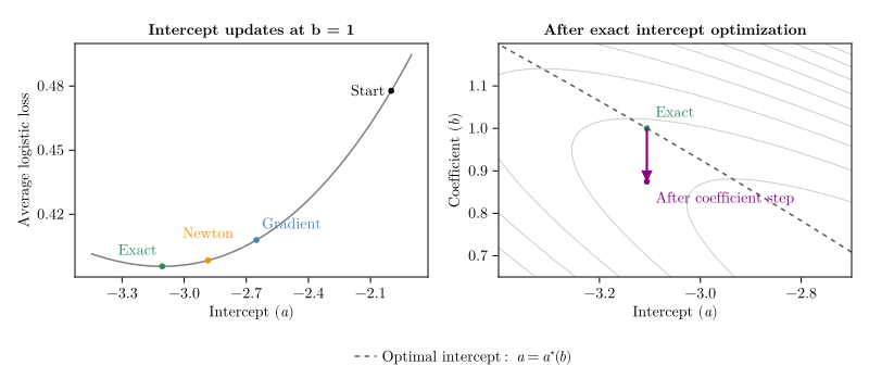
Figure 3 shows both the intercept updates and what happens after an exact solve. The optimal intercept depends on \(b\): changing the coefficient while holding the intercept fixed can move the iterate away from the curve \(a = a^\star(b)\). Thus, even exact intercept optimization need not give later coefficient updates in the same pass the profiled gradient.

let
    x = repeat([0.0, 1.0, 2.0]; inner = 10)
    y = zeros(30)
    y[[1, 11, 21, 22]] .= 1.0
    probability(a, b) = 1.0 ./ (1.0 .+ exp.(-(a .+ b .* x)))
    function objective(a, b)
        eta = a .+ b .* x
        return mean(max.(eta, 0.0) .+ log1p.(exp.(-abs.(eta))) .- y .* eta)
    end
    function optimal_intercept(b)
        # These endpoints bracket the root throughout the plotted range.
        lower, upper = -20.0, 20.0
        for _ in 1:60
            midpoint = (lower + upper) / 2
            if mean(probability(midpoint, b) .- y) > 0
                upper = midpoint
            else
                lower = midpoint
            end
        end
        return (lower + upper) / 2
    end

    a_start, b_start = -2.0, 1.0
    p_start = probability(a_start, b_start)
    g0 = mean(p_start .- y)
    h00 = mean(p_start .* (1 .- p_start))
    a_gradient = a_start - g0 / 0.25
    a_newton = a_start - g0 / h00
    a_exact = optimal_intercept(b_start)
    p_exact = probability(a_exact, b_start)
    gb = mean(x .* (p_exact .- y))
    hbb = mean(x.^2 .* p_exact .* (1 .- p_exact))
    b_next = b_start - gb / hbb

    fig = Figure(; size = output_size((800, 360)))
    ax_updates = Axis(
        fig[1, 1];
        title = "Intercept updates at b = 1",
        xlabel = L"Intercept ($a$)",
        ylabel = "Average logistic loss",
        xgridvisible = false,
        ygridvisible = false,
    )
    a_slice = range(-3.45, -1.9; length = 180)
    lines!(ax_updates, a_slice, objective.(a_slice, b_start); color = :gray50)
    for (a, label, color, offset, alignment) in [
            (a_start, "Start", :black, (-6, 0), (:right, :center)),
            (a_gradient, "Gradient", :steelblue, (5, 8), (:left, :bottom)),
            (a_newton, "Newton", :darkorange, (0, 18), (:center, :bottom)),
            (a_exact, "Exact", :seagreen, (-5, 8), (:right, :bottom)),
        ]
        scatter!(ax_updates, [a], [objective(a, b_start)]; color, markersize = 8)
        text!(
            ax_updates,
            a,
            objective(a, b_start);
            text = label,
            color,
            offset,
            align = alignment,
        )
    end

    ax_drift = Axis(
        fig[1, 2];
        title = "After exact intercept optimization",
        xlabel = L"Intercept ($a$)",
        ylabel = L"Coefficient ($b$)",
        xgridvisible = false,
        ygridvisible = false,
    )
    a_grid = range(-3.4, -2.7; length = 180)
    b_grid = range(0.65, 1.2; length = 180)
    values = [objective(a, b) for a in a_grid, b in b_grid]
    contour!(ax_drift, a_grid, b_grid, values; levels = 9, color = :gray80)
    lines!(
        ax_drift,
        optimal_intercept.(b_grid),
        b_grid;
        color = :gray35,
        linestyle = :dash,
        linewidth = 1.5,
    )
    scatter!(ax_drift, [a_exact], [b_start]; color = :seagreen, markersize = 8)
    text!(ax_drift, a_exact, b_start; text = "Exact", color = :seagreen, offset = (8, 8))
    arrows2d!(
        ax_drift,
        [a_exact],
        [b_start],
        [0.0],
        [b_next - b_start];
        color = :purple,
        shaftwidth = 2,
        tiplength = 10,
        tipwidth = 10,
    )
    scatter!(ax_drift, [a_exact], [b_next]; color = :purple, markersize = 8)
    text!(
        ax_drift,
        a_exact,
        b_next;
        text = "After coefficient step",
        color = :purple,
        offset = (8, -8),
        align = (:left, :top),
    )
    limits!(ax_drift, extrema(a_grid), extrema(b_grid))
    Legend(
        fig[2, 1:2],
        [LineElement(; color = :gray35, linestyle = :dash)],
        [L"Optimal intercept: $a = a^\star(b)$"];
        orientation = :horizontal,
        framevisible = false,
    )
    fig
end

Figure 3: Intercept updates for the logistic example in Equation 5. Left: the loss as a function of the intercept with \(b = 1\), showing the starting point and the three updated intercepts. Right: after exact intercept optimization, a coefficient Newton step with the intercept held fixed moves \(b\) from \(1\) to about \(0.875\) and decreases the loss, but leaves the curve of conditionally optimal intercepts. Gray curves are loss level sets. The right panel enlarges the neighborhood of the exact update.

To explain these differences for a general smooth loss, we expand the coefficient gradient after an intercept step. If we take the step \(\beta_0 \mapsto \beta_0 - \alpha \partial_0 F\), twice continuous differentiability gives \[ \partial_j F(\beta_0 - \alpha\partial_0 F, \beta) = \partial_j F(\beta_0, \beta) - \alpha H_{j0} \partial_0 F(\beta_0, \beta) + r_j(\alpha), \tag{6}\] where \(r_j(\alpha) = o(|d_0|)\) as the intercept displacement \(d_0 = -\alpha \partial_0 F\) tends to zero. If \(H_{j0}\) is locally Lipschitz, then \(r_j(\alpha) = O(d_0^2)\). For a quadratic objective, the gradient is affine, so the remainder is zero.

When \(H_{00} > 0\), the local Schur correction \(\partial_j F - (H_{j0}/H_{00})\partial_0 F\) is the gradient that a Newton intercept step predicts for the profiled objective at the current \(\beta\). It equals the profiled gradient in a frozen quadratic and approximates it locally for a nonlinear loss. Conditional minimization gives the true profiled gradient. The three strategies differ in how closely the gradient response in Equation 6 approaches that target.

3.3.3.1 What exact intercept optimization achieves

Exact minimization provides the reference for comparing the strategies. It gives the next coefficient update the profiled gradient, but the update still uses the curvature with the intercept held fixed. The following proposition makes this distinction precise.

Proposition 1 (First-update profile equivalence.) Let \(F\) be twice continuously differentiable and strictly convex in \(\beta_0\) for every \(\beta\), and let \(\tilde F(\beta) = \min_{\beta_0} F(\beta_0, \beta)\). Suppose the exact strategy has driven \(\beta_0\) to the conditional minimizer \(\beta_0^{(t)} = \arg\min_{\beta_0} F(\beta_0, \beta^{(t)})\), and suppose \(H_{00} > 0\) and \(\tilde H_{jj} > 0\) there. Then the first coefficient update of the next pass uses the gradient \(\partial_j F(\beta_0^{(t)}, \beta^{(t)}) = \partial_j \tilde F(\beta^{(t)})\), so its update direction agrees with the corresponding coordinate direction for \(\tilde F\) at \(\beta^{(t)}\). Its diagonal step size remains \(1/H_{jj}\). Because \(\tilde H_{jj} \leq H_{jj}\) by Equation 4, this step size is no larger than \(1/\tilde H_{jj}\), the step size for \(\tilde F\)’s local quadratic model along \(e_j\).

Proof. Let \(\beta_0^\star(\beta)\) be the conditional minimizer near \(\beta^{(t)}\). It exists at \(\beta^{(t)}\) by assumption and is unique by strict convexity. Since \(H_{00} > 0\) there, the implicit function theorem applied to \(\partial_0 F = 0\) makes \(\beta_0^\star\) differentiable locally. Thus \(\tilde F(\beta) = F(\beta_0^\star(\beta), \beta)\) near \(\beta^{(t)}\). Differentiating through \(\beta_0^\star\) and using the stationarity condition \(\partial_0 F(\beta_0^\star(\beta), \beta) = 0\), \[ \partial_j \tilde F(\beta) = \partial_j F(\beta_0^\star(\beta), \beta) + \partial_0 F\big(\beta_0^\star(\beta), \beta\big)\partial_j \beta_0^\star(\beta) = \partial_j F\big(\beta_0^\star(\beta), \beta\big). \] At the conditional minimizer, \(\partial_0 F = 0\), so the intercept’s dependence on \(\beta\) contributes nothing to the derivative. Evaluating at \(\beta_0^{(t)} = \beta_0^\star(\beta^{(t)})\) gives the gradient equality. For the step size, \(\tilde H_{jj} = H_{jj}(1 - \rho_{0j}^2) \leq H_{jj}\), so \(1/H_{jj} \leq 1/\tilde H_{jj}\) (Equation 4). The update therefore uses a step size no larger than the profiled local model’s \(1/\tilde H_{jj}\). This local comparison alone does not guarantee descent of \(\tilde F\) after a finite update.

The proposition establishes a gradient identity at the current coefficients. It does not turn a whole coordinate sweep into optimization of \(\tilde F\): the coefficient steps still use \(H_{jj}\), and later updates can move the intercept away from its conditional optimum. Before examining that drift, we ask how closely one Newton step reproduces the benefit of an exact solve.

3.3.3.2 How closely one Newton step matches an exact solve

A full Newton step leaves an intercept error that is quadratic in the current error, provided the curvature is positive and varies smoothly nearby. Write \(g(t) = \partial_0 F(t, \beta)\), let \(\beta_0^* = \beta_0^*(\beta)\) satisfy \(g(\beta_0^*) = 0\), and set \(H_{00} = g'(\beta_0)\). Taylor-expanding \(g(\beta_0^*)\) around the current iterate \(\beta_0\) gives \[ \partial_0 F(\beta_0, \beta) = H_{00}(\beta_0 - \beta_0^*) - \tfrac{1}{2}\partial_{000} F(\xi)(\beta_0 - \beta_0^*)^2, \tag{7}\] for some \(\xi\) between \(\beta_0\) and \(\beta_0^*(\beta)\). Dividing by \(H_{00}\) and recognizing \(\beta_0^{\text{Newton}} = \beta_0 - \partial_0 F/H_{00}\) on the left rewrites Equation 7 as the standard Newton identity for the iterate error: \[ \bigl|\beta_0^{\text{Newton}} - \beta_0^*(\beta)\bigr| = \frac{|\partial_{000} F(\xi)|}{2 |H_{00}|}(\beta_0 - \beta_0^*)^2. \tag{8}\] For a local bound, suppose that \(g'(t) \ge m > 0\) and \(|g''(t)| \le M\) between \(\beta_0\) and \(\beta_0^*\). The mean-value theorem gives \(m|\beta_0 - \beta_0^*| \le |g(\beta_0)|\), so Equation 8 yields \[ \bigl|\beta_0^{\text{Newton}} - \beta_0^*(\beta)\bigr| \le \frac{M}{2m^3} \bigl|\partial_0 F(\beta_0, \beta)\bigr|^2. \tag{9}\] Here we may take \(M\) as a bound on \(|\partial_{000}F| = |(1/n)\sum_i f'''(\eta_i)|\), and hence as no larger than \(\sup |f'''|\). For squared loss, \(f''' \equiv 0\) and the Newton step is exact. For logistic regression, \(|f'''|\) is bounded by a small constant. Thus, wherever the intercept curvature stays bounded away from zero, the residual shrinks quadratically as the current intercept gradient vanishes.

A small intercept error matters only through its effect on the coefficient update. We therefore carry this bound into the coefficient gradient. Let \(r_0 = \beta_0^{\text{Newton}} - \beta_0^*(\beta)\) be the Newton residual, with \(|r_0|\) bounded by Equation 9. Taylor-expanding \(\partial_j F\) in \(\beta_0\) around the conditional minimizer \(\beta_0^*(\beta)\), using \(\partial_j F(\beta_0^*, \beta) = \partial_j \tilde F(\beta)\) and \(H_{j0}^* = \partial_{0j} F(\beta_0^*, \beta)\), yields \[ \partial_j F\bigl(\beta_0^{\text{Newton}}, \beta\bigr) = \partial_j \tilde F(\beta) + H_{j0}^*r_0 + O(r_0^2), \tag{10}\] The coefficient gradient differs from the profiled gradient by \(b_j = H_{j0}^*r_0 + O(r_0^2)\). For a penalized problem, we also need to know how this difference changes the actual coordinate step. We isolate its effect by comparing both steps at the same positive curvature \(h_j\). Write \(G_\lambda(\beta) = \sum_j G_{\lambda,j}(\beta_j)\) and define the profiled step \[ d_j^{\mathrm{prof}} = \operatorname{prox}_{G_{\lambda,j}/h_j} \left( \beta_j - \frac{\partial_j\tilde F(\beta)}{h_j} \right) - \beta_j. \] The step \(d_j^{\mathrm{N}}\) after the Newton intercept update replaces \(\partial_j\tilde F\) by \(\partial_j\tilde F + b_j\). Nonexpansiveness of the proximal map gives \[ |d_j^{\mathrm{N}} - d_j^{\mathrm{prof}}| \leq \frac{|b_j|}{h_j}, \qquad |b_j| \ll h_j |d_j^{\mathrm{prof}}| \tag{11}\] as an absolute perturbation bound and a sufficient criterion for a small relative step error, respectively. The relevant comparison is with the composite coordinate residual \(h_j d_j^{\mathrm{prof}}\). At an active lasso optimum, \(\partial_j\tilde F = -\lambda\operatorname{sign}(\beta_j)\), so the smooth gradient itself generally does not vanish.

Under the local conditions of Equation 9, \(b_j\) is \(O(|\partial_0 F|^2)\) when the cross derivatives remain bounded. If \(h_j\) stays bounded away from zero, the profiled coordinate step remains first order in the iterate error, and \(\partial_0 F\) vanishes at least linearly, the Newton perturbation is second order and becomes negligible relative to that step. This is a conditional local comparison: when the profiled step is zero or vanishes faster, the absolute bound in Equation 11 still applies, but it supplies no relative guarantee.

Far from the optimum, the full-step approximation can fail when the third derivative is large, the intercept curvature approaches zero, or the intercept gradient is large. Poisson regression, where \(f''' = e^\eta\), can exhibit this cold-start behavior. Armijo backtracking safeguards descent, but a damped step has a different error bound from a full Newton step. With \(e_0 = \beta_0 - \beta_0^*(\beta)\) and accepted step fraction \(\alpha \in (0,1]\), the damped intercept error is \[ \beta_0^+ - \beta_0^*(\beta) = (1 - \alpha)e_0 + \alpha r_0. \tag{12}\] The quadratic error bound applies when the full step is accepted. For \(\alpha < 1\), sufficient decrease alone does not remove the first-order term \((1 - \alpha)e_0\).

The error bound and coupling correction describe a single Newton step at the current iterate (Equation 9–Equation 10). The experiments in Section 4 show how those gains accumulate across an outer solve.

3.3.3.3 What a gradient step leaves behind

The gradient strategy uses the curvature bound \(L_0\) in place of the current intercept curvature \(H_{00}\). Its step can therefore be much smaller than the Newton step. When \(H_{00} > 0\), substituting \(\alpha = 1/L_0\) into Equation 6 gives \[ \partial_j F^{\text{grad}} = \partial_j F - \frac{H_{00}}{L_0}\frac{H_{j0}}{H_{00}}\partial_0 F + r_j(1/L_0), \tag{13}\] so, to first order, the gradient strategy removes a fraction \(H_{00}/L_0 \in (0, 1]\) of the coupling component \((H_{j0}/H_{00})\partial_0 F\) that Newton targets at leading order. The exact strategy instead reaches the true profiled gradient by conditional minimization. In a frozen quadratic, \(r_j(1/L_0) = 0\) and the correction fraction is exact. For a nonlinear loss, the leading-order residual relative to the local Schur-corrected target is \((1 - H_{00}/L_0)(H_{j0}/H_{00})\partial_0 F + r_j(1/L_0)\). When \(L_0 = \infty\), the intercept step is zero, so no coupling is removed.

The leading-order correction is fully effective only when \(H_{00} \approx L_0\), that is, when the Lipschitz bound is tight at the current iterate. Whenever \(H_{00}\) is appreciably below \(L_0\)—as happens for logistic regression once predictions become confident, or whenever the weights \(w_i\) are concentrated on a small subset of observations—the gradient strategy leaves a fraction \(1 - H_{00}/L_0\) of the leading-order coupling correction unapplied. The remaining intercept error continues to affect the coefficient gradients and can slow subsequent passes.

For Poisson loss, this strategy has no finite global curvature bound to use: \(L_0 = \infty\) gives a zero intercept step at every finite iterate. The coefficient gradients then retain the full effect of the intercept error. This limitation concerns the strategy based on a global bound; a gradient method with an adaptive step size or line search need not leave the intercept fixed.

3.3.3.4 Why extra intercept iterations may not pay off

The comparisons above hold the coefficients fixed. During a coordinate sweep, however, each coefficient update can move the intercept’s conditional optimum. Even an exact intercept solve therefore guarantees the profiled gradient only for the first coefficient update of the next pass.

To measure this drift, expand \(\partial_0 F\) in the \(\beta_j\) direction at the conditional minimizer. With \(\partial_{0j} F = H_{0j}\) and \(\partial_0 F(\beta_0^{(t)}, \beta^{(t)}) = 0\), a single coefficient update \(\beta_j^{(t)} \mapsto \beta_j^{(t)} + \delta_j\) gives, when the relevant Hessian entries are locally Lipschitz, \[ \partial_0 F \big(\beta_0^{(t)}, \beta^{(t)} + \delta_j e_j \big) = H_{0j}\delta_j + O(\delta_j^2). \tag{14}\] When this change is nonzero, the intercept is no longer conditionally optimal, and Proposition 1 no longer guarantees the profiled gradient for the next coefficient update. The drift depends on both the coupling and the coefficient step; it need not occur after every update.

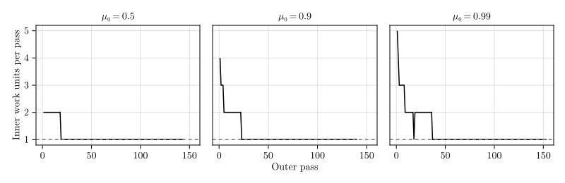
The exact strategy spends extra work optimizing an intercept that the next coefficient update may immediately move away from its optimum. Let \(k_0\) count the inner work units needed at the end of a pass to reach \(|\partial_0 F| < \varepsilon\), including one residual check when the intercept already meets this tolerance. Across the imbalance levels in our experiments, \(k_0\) ranged from one to five, with each unit costing \(O(n)\) work (Figure 29). With the coefficients held fixed, Newton’s method converges rapidly near the intercept’s conditional minimizer: under its usual local convergence conditions, reaching tolerance \(\varepsilon\) requires \(O(\log\log(1/\varepsilon))\) further iterations. This rate does not account for the work needed to enter that neighborhood, nor does it guarantee that the intercept starts there after each coefficient pass.

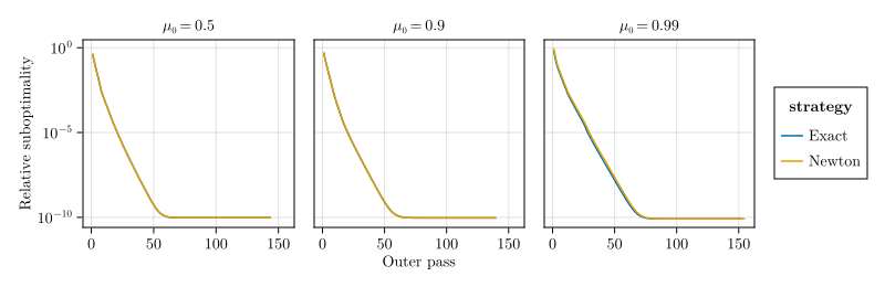
Together, the Newton error bound and the drift calculation explain why one Newton step can be enough: locally, it leaves only a second-order intercept error, while the next coefficient update can introduce fresh error even after an exact solve. These calculations do not establish how much the extra inner iterations affect convergence over a full solve. The experiments in Supplement S4.3 supply that comparison: on our test problems, the additional work produces little improvement in outer convergence.

The tradeoff can differ in other settings. Along a warm-started \(\lambda\) path, a small initial intercept gradient can reduce \(k_0\) to one or two work units, leaving little overhead for the exact strategy. Strong coupling makes any remaining intercept error more consequential for the coefficient gradients (Equation 10), but it also increases the drift caused by coefficient updates (Equation 14). Coupling alone therefore does not determine whether extra intercept iterations are worthwhile.

IRLS and prox-Newton methods also require a separate comparison because they update the coefficients through a quadratic surrogate. With the coefficients fixed, one full Newton step solves that surrogate’s intercept subproblem exactly. Updating the coefficients can still move its optimal intercept, and rebuilding the surrogate does not by itself eliminate this drift. LIBLINEAR resolves the intercept within its frozen quadratic, whereas BlitzL1 applies an exact-strategy loop to the original loss after the prox-Newton step (Section 3.4). The cost and benefit depend on where these solves occur in the outer algorithm. Our recommendation to avoid extra intercept iterations concerns the cold-start, direct-CD experiments studied here; it is not a general claim about these other settings.

3.3.4 Local-rate interpretation

To follow the correction in Equation 13 through successive passes, we study a local quadratic model. For the lasso, freeze the Hessian at the optimum and restrict the coefficients to the active set \(A\) with their signs fixed. Assume this restricted Hessian is positive definite and define the collective coupling \[ \kappa = \frac{H_{0A}H_{AA}^{-1}H_{A0}}{H_{00}} \in [0, 1). \tag{15}\] If each pass first minimizes the active coefficient block and then updates the intercept, Newton contracts the intercept error by \(\kappa\), whereas the gradient strategy contracts it by \(1 - (H_{00}/L_0)(1 - \kappa)\). As \(\kappa \to 1\), the ratio of the required pass counts approaches \(L_0/H_{00}\). Thus, coupling determines when the intercept mode controls convergence, and the curvature ratio determines how much slower the gradient strategy becomes once it does.

This is a local explanation, not a global iteration-complexity theorem. A coordinate sweep retains coefficient error modes that the exact block solve eliminates. Supplement S1.1 gives the block calculation and validates the full frozen coordinate-sweep model against nonlinear convergence rates. The centering experiment there varies coupling while holding the intercept curvature fixed, exposing the transition to the \(L_0/H_{00}\) plateau.

3.3.5 A safe Newton variant

The Newton-coupling bias (Equation 10) identifies the cold-start regime—large \(|\partial_0 F|\) combined with rapidly varying \(f''\)—as the setting where an unguarded Newton step on the intercept perturbs the next coefficient pass enough to matter. The fix is to wrap the Newton direction \(-\partial_0 F / H_{00}\) in an Armijo backtracking line search: accept the full step (\(\alpha = 1\)) if it decreases \(F\) enough. Otherwise, halve \(\alpha\) until it does. Our Newton strategy includes this safeguard. When it accepts the full step, the safeguard adds constant work; when the linear model is inadequate, the number of backtracking trials grows logarithmically. To isolate the effect of the guard, we compare the guarded variant directly with a bare Newton step in Figure 7 and Figure 8 and show when the guard changes the result.

3.3.6 Extension to vector intercepts

The same mechanism extends to multinomial logistic regression. Under a reference-class parameterization, the intercept becomes a \((K - 1)\)-vector, and its Hessian is \[ H_{00} = \frac{1}{n}\sum_{i=1}^n \left\{ \operatorname{diag}(p_{i,1:K-1}) - p_{i,1:K-1}p_{i,1:K-1}^{\top} \right\}. \] Rare free classes create low-curvature coordinate directions. A rare reference class creates a low-curvature common-shift direction. A global Böhning majorant therefore attenuates the intercept correction in precisely the modes associated with rare classes. A single Armijo-guarded Newton block step adapts to those modes, while the exact strategy adds inner iterations without a visible improvement in the outer trajectory. Supplement S2.1 derives the block update, identifies the relevant Rayleigh quotients, and tests this prediction on a grid of synthetic problems.

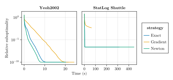
The pattern appears on two real datasets with contrasting dimensions (Figure 4). Yeoh2002 has \(n = 248\), \(p = 12\,625\), and six classes, while StatLog Shuttle has \(n = 58\,000\), \(p = 9\), and seven classes. We set \(\lambda = 0.05\lambda_{\max}\) in both problems, where \(\lambda_{\max}\) is the smallest penalty for which all fitted slopes are zero.

On Yeoh2002, the gradient strategy needs roughly four times as many passes as Newton to bring the relative suboptimality bound below \(10^{-4}\). On Shuttle, whose rarest classes contain only ten and thirteen observations, it fails to reach \(10^{-4}\) within 1,000 passes; Newton and exact reach that threshold in \(20\)–\(21\) passes.

dd_yeoh = JLD2.load(@projectroot("results", "real-multinomial-yeoh.jld2"))
df_yeoh = DataFrame(dd_yeoh["results"])
df_yeoh = flatten(df_yeoh, [:time, :relgaps, :gaps, :primals])
df_yeoh.dataset = fill("Yeoh2002", nrow(df_yeoh))

dd_shuttle = JLD2.load(@projectroot("results", "real-multinomial-shuttle.jld2"))
df_shuttle = DataFrame(dd_shuttle["results"])
df_shuttle = flatten(df_shuttle, [:time, :relgaps, :primals])
df_shuttle.dataset = fill("StatLog Shuttle", nrow(df_shuttle))

df_multinomial = vcat(
    select(df_yeoh, :time, :relgaps, :strategy, :dataset),
    select(df_shuttle, :time, :relgaps, :strategy, :dataset),
)
df_multinomial.relgaps .= max.(df_multinomial.relgaps, 1.0e-10)
df_multinomial.strategy = strategy_label.(df_multinomial.strategy)

draw(
    visual(Lines) *
        data(df_multinomial) *
        mapping(
            :time => "Time (s)",
            :relgaps => "Relative suboptimality",
            color = :strategy,
            col = :dataset => sorter("Yeoh2002", "StatLog Shuttle"),
        ),
    axis = (yscale = log10,),
    facet = (; linkxaxes = false),
    figure = (; size = output_size((600, 280))),
)

Figure 4: Multinomial logistic regression on two real datasets. The panels show a relative suboptimality bound versus time for Yeoh2002 (\(p \gg n\)) and StatLog Shuttle (\(n \gg p\)) at \(\lambda = 0.05\lambda_{\max}\) under cyclic coordinate descent.

3.4 Connection to IRLS

So far, we have considered direct coordinate descent on \(F\), which recomputes the weights \(w_i = f''(\eta_i; y_i)\) after every coefficient update. A widely used alternative—and the one used by glmnet (Friedman et al. 2010)—is iteratively reweighted least squares (IRLS) (McCullagh and Nelder 1989). At the current iterate \((\beta_0^{(t)}, \beta^{(t)})\), IRLS forms the weighted least squares quadratic surrogate \[ \tilde F^{(t)}(\beta_0, \beta) = \frac{1}{2n} \sum_{i=1}^n w_i^{(t)} \bigl( z_i^{(t)} - \beta_0 - x_i^\top \beta \bigr)^2, \] with working response \(z_i^{(t)} = \eta_i^{(t)} - r_i^{(t)} / w_i^{(t)}\). It then solves \(\tilde F^{(t)}\) by inner CD and re-linearizes. In practice, solvers use two kinds of weights: local weights \(w_i^{(t)} = f''(\eta_i^{(t)}; y_i)\) (glmnet’s type.logistic = "Newton"), and MM-majorized weights replacing \(w_i^{(t)}\) by a global upper bound on \(f''\) (e.g., \(w_i \equiv 1/4\) for logistic regression, as in glmnet’s type.logistic = "modified.Newton", following the MM tradition of Hunter and Lange (2004)).

Within an inner solve with local weights, \(\tilde F^{(t)}\) is quadratic in \(\beta_0\) with curvature \((1/n)\sum_i w_i^{(t)} = H_{00}\), so the inner Lipschitz constant satisfies \(L_0^{\text{inner}} = H_{00}\). The fraction in Equation 13 is therefore \(H_{00} / L_0^{\text{inner}} = 1\). Because a Newton step on a quadratic is exact, the gradient, Newton, and exact strategies all coincide on the inner subproblem. Thus, the distinction that we analyze is specific to direct-CD solvers, such as skglm, and does not arise within a local-weight IRLS inner solve.

The strategies no longer coincide under MM majorization. Replacing \(w_i^{(t)}\) by the constant majorant \(1/4\) in the logistic case, the closed-form inner intercept update on \(\tilde F^{(t)}\) is \[ \beta_0 \gets \beta_0 + \frac{4}{n} \sum_{i=1}^n (y_i - p_i) = \beta_0 - \frac{1}{L_0} \partial_0 F, \qquad L_0 = 1/4, \] which is the gradient strategy with a global Lipschitz step. The identity holds at the linearization point, where \(p_i\) is evaluated, so it describes the first inner intercept update after each re-linearization; once inner CD has moved \(\beta\), subsequent inner updates drive the intercept to the conditional minimum of the frozen majorant quadratic (Table 3) rather than taking further \(1/L_0\) steps on the original loss.

The correction transmitted at each re-linearization is nevertheless governed by the same attenuation. The Schur-coupling residual (Equation 13) thus applies directly to glmnet’s modified.Newton mode: under response imbalance, the leading-order correction fraction \(H_{00}/L_0\) shrinks and the intercept update slows, approaching a true stall only as fitted probabilities reach the boundary.

MM majorization was introduced to stabilize the working response \(z_i\) when \(w_i \to 0\)—the same regime in which the resulting update converges slowly. For Poisson loss, no global upper bound on \(f''\) exists, so this MM construction is unavailable. glmnet instead uses local-weight IRLS, where the three strategies coincide as described above.

Changing from local weights to the constant majorant also changes every coefficient’s curvature and cross-curvature in the surrogate. A within-package mode comparison therefore isolates the IRLS weight scheme, not the intercept update alone. The intercept correction is the component of that scheme analyzed by Equation 13; Figure 16 compares changes to intercept handling within a direct-CD solver.

Across IRLS linearizations, the weights \(w_i^{(t)}\) change with \(\eta^{(t)}\), so even a fully resolved inner intercept becomes stale once the weights are recomputed. This outer-level drift is analogous to but distinct from the within-pass drift of Equation 14, which is specific to direct CD.

The appropriate intercept strategy therefore depends on the solver family. The production solvers fall into the classes in Table 3. Of the CD-based packages that we surveyed, only skglm 0.5 and earlier apply a conservative gradient update directly to the original loss. The remaining solvers—glmnet, biglasso, adelie, LIBLINEAR, BlitzL1, Lasso.jl, and ncvreg (Breheny and Huang 2011)—all linearize before running CD, using either IRLS or proximal-Newton (Lee et al. 2014) on a quadratic upper bound.⁵ The mode switches within glmnet (Newton versus modified.Newton) and biglasso (Newton versus MM) isolate the effect of the weight scheme analyzed in Equation 13.

We exclude two related implementations from the table. Scikit-learn’s L1-logistic path either delegates to LIBLINEAR or uses SAGA, a variance-reduced stochastic-gradient method outside the CD framework analyzed here. celer’s L1-logistic estimator does not support an intercept in version 0.7.4, and its documentation directs users to skglm for logistic regression.

Table 3: Classification of CD-based production solvers by algorithmic family and intercept treatment. IRLS and prox-Newton rows conditionally minimize a frozen quadratic surrogate, not the original GLM loss; BlitzL1 alone additionally applies a post-step one-dimensional Newton loop on the original loss.

Solver	Family	Intercept treatment
skglm 0.5	Constant-Lipschitz CD	Gradient on original loss (step size \(1/4\))
glmnet (type.logistic = "modified.Newton")	MM-IRLS	Conditional minimum of global-majorant quadratic
biglasso (alg.logistic = "MM")	MM-IRLS	Conditional minimum of global-majorant quadratic
glmnet (type.logistic = "Newton")	Local-IRLS	Conditional minimum of frozen local quadratic
biglasso (alg.logistic = "Newton", default)	Local-IRLS	Conditional minimum of frozen local quadratic
adelie	Local-IRLS	Conditional minimum of weighted, centered quadratic
LIBLINEAR (newGLMNET, L1-LR)	Prox-Newton	Conditional minimum of frozen quadratic; unregularized
BlitzL1	Prox-Newton	Post-step Newton convergence on original loss

LIBLINEAR (newGLMNET) and BlitzL1 treat the intercept differently at the boundary of each prox-Newton step. LIBLINEAR leaves the intercept unregularized inside the inner CD solve. As the quadratic program converges, the intercept reaches the conditional minimum of the frozen quadratic, which generally differs from that of the original loss. BlitzL1 additionally runs an explicit one-dimensional Newton loop to convergence on the original loss after each subproblem and therefore applies the exact strategy at that boundary.

The within-pass drift of Equation 14 penalizes the exact strategy within direct CD because the inner Hessian drifts between iterations. That critique does not apply at the prox-Newton boundary, where the next subproblem’s Hessian is recomputed anyway.

For direct CD, we therefore recommend a Newton update of the intercept. Within each IRLS or prox-Newton quadratic surrogate, we recommend optimizing the intercept fully, with an optional correction on the original loss at the linearization boundary. The surveyed production solvers follow the first two recommendations; BlitzL1 also follows the third.

In Figure 5, we compare direct CD and IRLS on a synthetic logistic problem. Throughout the synthetic experiments, \(\mu_0\) denotes the baseline mean response at \(x = 0\)—a positive-class probability for binomial models and a rate for Poisson models—and \(s\) is the number of nonzero slopes in each generated coefficient vector. Once the slopes enter the linear predictor, \(\mu_0\) need not equal the empirical response mean.

dd = JLD2.load(@projectroot("results", "sim-irls-comparison.jld2"))
df = DataFrame(dd["results"])
df = flatten(df, [:time, :relgaps, :gaps, :primals])

df.relgaps .= max.(df.relgaps, 1.0e-10)
df.it = "seed = " .* string.(df.it)

spec = data(df) * mapping(:time, :relgaps, color = :strategy, col = :it)

draw(
    visual(Lines) * spec,
    axis = (yscale = log10, ylabel = "Relative suboptimality", xlabel = "Time (s)"),
    facet = (; linkxaxes = :none),
    figure = (; size = output_size((800, 250))),
)

Figure 5: Direct CD and IRLS on an imbalanced logistic design. The panels show a relative suboptimality bound versus time for \(\mu_0 = 0.99\), \(n = 500\), \(p = 1000\), \(s = 10\), \(\lambda = 0.05\lambda_{\max}\), and three random seeds. The Local-IRLS curve is shown once because the three intercept strategies coincide on the inner quadratic.

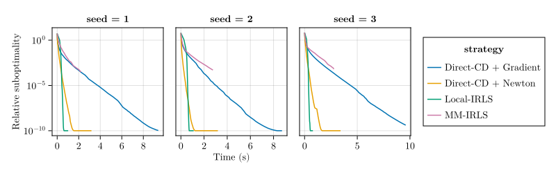
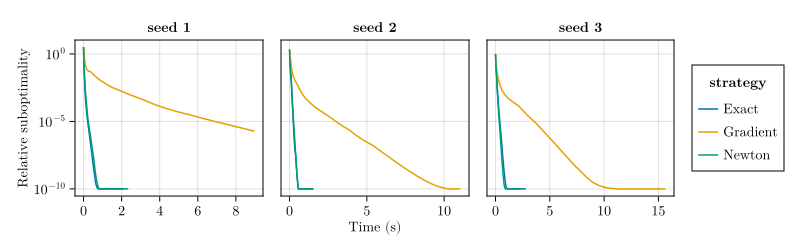
Local-IRLS converges fastest under \(\mu_0 = 0.99\), crossing the \(10^{-8}\) bound in about 25 passes across the three seeds (Figure 5). Direct-CD with Newton takes roughly twice as many passes, while Direct-CD with the gradient strategy takes several hundred. MM-IRLS remains above \(10^{-4}\) after 200 passes. Within Local-IRLS, the three strategies coincide exactly: once \(L_0^{\text{inner}} = H_{00}\), they share the single inner update \(-\partial_0 \tilde F^{(t)} / H_{00}\) and produce identical iterates. The figure therefore plots only one curve. Unit tests verify exact agreement of the intercept and coefficient paths.

Local-IRLS also outpaces Direct-CD with the Newton strategy on this problem. This difference concerns the two algorithmic families rather than their intercept strategies: IRLS-CD uses a constant inner Hessian and has locally quadratic outer convergence, which favors it on canonical-link GLMs where the linearization is tight. Direct-CD has the edge when \(f'''\) is large (e.g.
Poisson with extreme rates, where each linearization is loose far from the current iterate), when saturation makes the working response unstable, or when screening and working-set methods (standard in modern \(\ell_1\) solvers) work poorly with re-linearization (Bertrand et al. 2022). This family-level difference does not change the intercept recommendation: within either family, use local Newton curvature rather than a global Lipschitz bound.

4 Results

4.1 Methodology and reproducibility

We run the internal experiments using our Julia implementations of the solvers and report outer passes as the primary measure of work. Unless otherwise noted, synthetic designs use cyclic ordering, fixed seeds, standardized features, and an AR(1) correlation of \(\rho = 0.6\). We evaluate comparable trajectories against the strongest feasible dual value found for their shared problem instance, so the displayed suboptimality bound does not depend on which strategy produced the primal iterate. We use pinned datasets in the real-data experiments and follow the same shared-reference principle in the production comparison. We load cached outputs for computationally expensive experiments. The toy examples in Figure 1 and Figure 3 run when the notebook renders. We pin the Julia, R, and Python environments in the repository and document the problem construction, tolerances, budgets, data preparation, hardware, and reproduction protocol in Supplement S3.

4.2 Simulated data

We begin with the simplest consequence of Section 3. The gradient strategy’s intercept step is the local Newton direction scaled by \(H_{00}/L_0\). As imbalance pushes \(\mu_0\) toward one, \(H_{00}\) shrinks while \(L_0 = 1/4\) remains fixed. We therefore expect the intercept update to slow.

4.2.1 Synthetic trajectories and safeguards

We compare the strategies on a standardized binary-logistic design with \(n = 500\), \(p = 1000\), \(s = 10\), AR(1) correlation \(\rho = 0.6\), cyclic CD, and \(\lambda = 0.05\lambda_{\max}\).

dd = JLD2.load(@projectroot("results", "sim-mu-extreme.jld2"))
df = DataFrame(dd["results"])
df = flatten(df, [:time, :relgaps, :gaps, :primals])

df.relgaps .= max.(df.relgaps, 1.0e-10)
df.strategy = strategy_label.(df.strategy)
df.μ0 = [L"$\mu_0 = %$(v)$" for v in df.μ0]

spec = data(df) * mapping(:time, :relgaps, color = :strategy, col = :μ0)

draw(
    visual(Lines) * spec,
    axis = (yscale = log10, ylabel = "Relative suboptimality", xlabel = "Time (s)"),
    facet = (; linkxaxes = :none),
    figure = (; size = output_size((800, 250))),
)

Figure 6: Imbalance sweep on the standardized logistic design. The panels show a relative suboptimality bound versus time for the intercept-update variants in the legend as \(\mu_0\) varies, with \(n = 500\), \(p = 1000\), \(s = 10\), \(\lambda = 0.05\lambda_{\max}\), and cyclic CD.

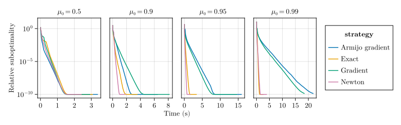
The Schur-coupling residual (Equation 13) predicts that the gradient strategy will slow as \(H_{00}/L_0\) approaches zero when \(\mu_0\) approaches one. At \(\mu_0 = 0.99\), the gradient strategy needs about fifteen times as many passes as Newton to reach \(10^{-8}\) in our experiment, whereas the Newton and exact strategies remain close across the sweep (Figure 6). Their agreement supports the prediction that exact profiling adds little progress in the outer solve beyond one Newton step (Equation 14); Supplement S4.3 compares their inner work.

dd = JLD2.load(@projectroot("results", "sim-cold-start.jld2"))
df = DataFrame(dd["results"])
df = flatten(df, [:time, :relgaps, :gaps, :primals])

df.relgaps .= max.(df.relgaps, 1.0e-10)
df.strategy = strategy_label.(df.strategy)
df.μ0 = [L"$\mu_0 = %$(v)$" for v in df.μ0]

spec = data(df) *
    mapping(:time, :relgaps, color = :strategy, col = :μ0, group = :it => nonnumeric)

draw(
    visual(Lines, alpha = 0.6) * spec,
    axis = (yscale = log10, ylabel = "Relative suboptimality", xlabel = "Time (s)"),
    facet = (; linkxaxes = :none),
    figure = (; size = output_size((800, 250))),
)

Figure 7: Logistic cold-start comparison. The panels show a relative suboptimality bound versus time for bare Newton, Armijo-guarded Newton, and the exact strategy across the \(\mu_0\) levels of Figure 6. Each panel shows five simulated replicates per strategy.

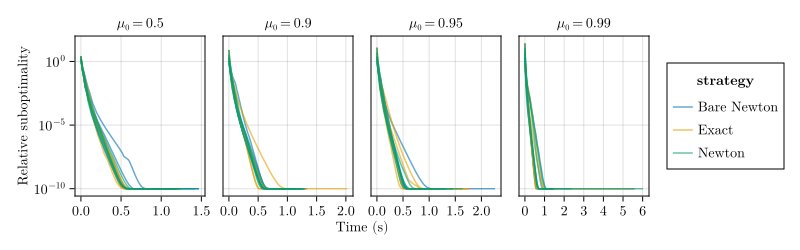
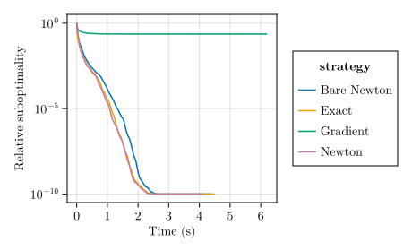
The Newton-coupling bias (Equation 10) leads to a second prediction: at a cold start, a large \(|\partial_0 F|\) can make an unguarded Newton step on the intercept unstable. To test this prediction directly, we run bare Newton (without Armijo backtracking) alongside the guarded variant and the exact strategy in Figure 7.

For logistic regression, the three trajectories are indistinguishable, even in the most imbalanced case at \(\mu_0 = 0.99\). The Armijo guard rarely activates: most guarded runs are identical bit for bit to their bare Newton counterparts, and the remaining pairs begin to differ only late in the solve, never at cold start. Every guarded and bare Newton pair crosses the shared \(10^{-8}\) bound on the same pass. The exact strategy differs from them by only a handful of passes.

Thus, the Armijo safeguard does not improve the logistic cold starts tested here: the full Newton step is accepted at the initial iterate, and the few later differences do not systematically favor either variant. Logistic curvature is bounded, \(f'' = \mu(1 - \mu) \le 1/4\), but bounded curvature alone does not guarantee that an undamped Newton step decreases the objective at every iterate. These experiments establish the narrower empirical result for the zero-initialized problem family above.

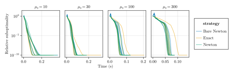
Losses with unbounded curvature behave differently. For Poisson regression with the canonical log link, \(f''(\eta) = e^\eta\) and \(f'''(\eta) = e^\eta\) both grow without bound, so the Newton linearization is loose far from the optimum and the unguarded step can overshoot by an arbitrary factor. We repeat the cold-start experiment on synthetic Poisson data with \(n = 500\), \(p = 1000\), \(s = 10\), \(\lambda = 0.1\lambda_{\max}\), and baseline rates \(\mu_0 \in \{10, 30, 100, 300\}\).

dd_p = JLD2.load(@projectroot("results", "sim-cold-start-poisson.jld2"))
df_p = DataFrame(dd_p["results"])
df_p = flatten(df_p, [:time, :relgaps, :gaps, :primals])

df_p.relgaps .= max.(df_p.relgaps, 1.0e-10)
df_p.strategy = strategy_label.(df_p.strategy)
μ0_levels = [L"$\mu_0 = %$(Int(m))$" for m in sort(unique(df_p.μ0))]
df_p.μ0 = [L"$\mu_0 = %$(Int(m))$" for m in df_p.μ0]

spec_p = data(df_p) *
    mapping(
        :time,
        :relgaps,
        color = :strategy,
        col = :μ0 => sorter(μ0_levels),
        group = :it => nonnumeric,
    )

draw(
    visual(Lines, alpha = 0.6) * spec_p,
    axis = (
        yscale = log10,
        ylabel = "Relative suboptimality",
        xlabel = "Time (s)",
        xticks = WilkinsonTicks(3),
    ),
    facet = (; linkxaxes = :none),
    figure = (; size = output_size((800, 250))),
)

Figure 8: Poisson cold-start comparison. The panels show a relative suboptimality bound versus time for bare Newton, Armijo-guarded Newton, and the exact strategy at baseline rates \(\mu_0 \in \{10, 30, 100, 300\}\), with \(n = 500\), \(p = 1000\), \(s = 10\), and \(\lambda = 0.1\lambda_{\max}\). Each panel shows five simulated replicates per strategy.

At \(\mu_0 = 300\), the first bare Newton step moves the cold-start intercept from zero to \(\bar{y} - 1 \approx 300\), although the intercept-only optimum is only \(\log(\bar{y}) \approx 6\). Because the log link exponentiates the intercept, this step implies a fitted rate near \(e^{300}\) and makes the loss astronomical at that intermediate iterate. The safeguard prevents this overshoot (Figure 8): the unguarded bound jumps several-fold after the first pass, while the guarded bound falls immediately.

The overshoot is nonetheless recoverable. The outer CD loop’s own per-coordinate Armijo guard absorbs it over the next few passes, and the final primal values agree to numerical precision. The three strategies return to nearly the same trajectory within a few passes.

The guard therefore keeps the iterates numerically reasonable but provides no visible improvement in the convergence rate here. The exact strategy is competitive in both experiments but incurs the cost of within-pass drift identified in Equation 14. It applies the same Armijo safeguard to every inner Newton direction. Every returned scalar update satisfies \(|\partial_0 F| \le 10^{-10}\). Reaching the iteration cap would stop the experiment before the result could be cached.

4.3 Real data

We next examine whether the same scaling appears on real problems. We run the three strategies on six LIBSVM benchmark problems at \(\lambda = 0.05\lambda_{\max}\). Table 4 lists the problems in order of the reciprocal intercept-only curvature fraction \([4 \pi_+ (1 - \pi_+)]^{-1}\). The table lists the curvature fraction itself, \(4 \pi_+ (1 - \pi_+)\). The six problems span a ninefold range in this quantity and include sparse and dense designs in both dimensional regimes.

The two most imbalanced problems, w1a and news20-3pct, are especially useful. They have nearly the same \(\pi_+\) but very different sparse designs: w1a has 300 web-indicator features, while news20-3pct is drawn from a text corpus with an original vocabulary of roughly \(1.3\) million terms and retains 4,675 features after filtering. Agreement between them would suggest that the slowdown is not peculiar to w1a.

Table 4: LIBSVM problems used in Figure 9. \(\pi_+\) is the positive-class marginal, and \(4\pi_+(1 - \pi_+)\) is the intercept-only curvature fraction, not the fitted \(H_{00}/L_0\). news20-3pct is a deterministic 60/1,940 subsample of news20.binary; after subsampling, features with fewer than 20 nonzeros are dropped.

dataset	\(n\)	\(p\)	density	\(\pi_+\)	\(4\pi_+(1 - \pi_+)\)
w1a	2,477	300	sparse	0.029	0.113
news20-3pct	2,000	4,675	sparse	0.030	0.116
a4a	4,781	123	sparse	0.248	0.747
leukemia	38	7,129	dense	0.711	0.823
breast-cancer	683	10	dense	0.350	0.910
gisette	6,000	5,000	dense	0.500	1.000

dd = JLD2.load(@projectroot("results", "real-logreg.jld2"))
df = DataFrame(dd["results"])
df = flatten(df, [:time, :relgaps, :gaps, :primals])

df.relgaps .= max.(df.relgaps, 1.0e-10)
df.strategy = strategy_label.(df.strategy)
df.dataset = replace.(
    df.dataset,
    "gisette_scale" => "gisette",
    "news20-imb" => "news20-3pct",
)

dataset_order = ["w1a", "news20-3pct", "a4a", "leukemia", "breast-cancer", "gisette"]

spec = data(df) *
    mapping(
        :time => "Time (s)",
        :relgaps => "Relative suboptimality",
        color = :strategy,
        layout = :dataset => sorter(dataset_order...),
    )

draw(
    visual(Lines) * spec,
    axis = (yscale = log10,),
    facet = (; linkxaxes = :none),
    figure = (; size = output_size((800, 500))),
)

Figure 9: Real-data logistic convergence on six LIBSVM problems. The panels show a relative suboptimality bound versus time for the three intercept strategies at \(\lambda = 0.05\lambda_{\max}\), in the problem order of Table 4.

The two severely imbalanced datasets reproduce both predicted patterns on very different sparse designs. The gradient strategy takes about six times as many passes as Newton to reach \(10^{-6}\) on w1a and about ten times as many to reach \(10^{-4}\) on news20-3pct, before the latter reaches its wall-time cap. Both datasets have small intercept-only curvature fractions. Their large slowdowns across different designs support the response-imbalance mechanism, although the fitted curvature and collective coupling determine the local rate.

For the moderately imbalanced a4a and breast-cancer data, the gap between the gradient and Newton strategies is modest—less than threefold—consistent with their larger intercept-only curvature fractions. Leukemia (\(n \ll p\), penalty-dominated) and gisette (dense and balanced) serve as negative controls: leukemia shows little separation, and the gisette pass counts are identical. The exact strategy tracks Newton on every panel, consistent with Equation 14 at this tolerance.

Poisson data offer a sharper version of the same test. The Poisson loss has no global upper bound on \(f''(\eta) = e^\eta\), so \(L_0 = \infty\) and the gradient-strategy update degenerates: the per-pass change is \(-\sum_i (\hat\mu_i - y_i)/(L_0 n) = 0\), so the intercept remains unchanged. We test this on the congress109 phrase-count corpus of Taddy (2015).

The corpus contains \(n = 529\) speakers from the 107th–109th US Congress and \(p = 999\) political phrases (the 1,000-phrase vocabulary with the response phrase removed). The response \(y_i\) is speaker \(i\)’s count of the phrase american.people (\(\bar y = 11.83\), \(y_{\max} = 396\)), the highest-frequency phrase in the corpus. The features are the remaining \(999\) phrase counts after column standardization.

This setup follows the construction for distributed multinomial regression in Taddy (2015), which approximates a multinomial model over the vocabulary by fitting an independent Poisson lasso for each term. The baseline rate \(\bar y \approx 12\) places the problem near the beginning of the synthetic cold-start sweep in Figure 8 (\(\mu_0 = 10\)). At this rate, the first bare Newton step is \(\bar y - 1 \approx 10.83\), while the intercept-only optimum is \(\log(\bar y) \approx 2.47\). We set \(\lambda = 0.05\lambda_{\max}\) and use cyclic CD with a \(1\,000\)-pass budget.

dd = JLD2.load(@projectroot("results", "real-poisson.jld2"))
df = DataFrame(dd["results"])
df = flatten(df, [:time, :relgaps, :gaps, :primals])
df.relgaps .= max.(df.relgaps, 1.0e-10)
df.strategy = strategy_label.(df.strategy)

spec = data(df) *
    mapping(:time => "Time (s)", :relgaps => "Relative suboptimality", color = :strategy)
draw(
    visual(Lines) * spec,
    axis = (yscale = log10,),
    figure = (; size = output_size((460, 280))),
)

Figure 10: Poisson regression on congress109. The plot shows a relative suboptimality bound versus time for the four intercept strategies at \(n = 529\), \(p = 999\), \(\bar y = 11.83\), and \(\lambda = 0.05\lambda_{\max}\).

In Figure 10, the gradient strategy leaves the intercept unchanged because \(L_0 = \infty\). This failure follows from the loss family rather than from tuning or a problem-specific imbalance level. Newton and exact follow the same trajectory because the CD solver’s per-coordinate Armijo loop (Tseng–Yun sufficient decrease, Algorithm 1) absorbs the cold-start overshoot before the first intercept update occurs. The synthetic suboptimality curves expose the unguarded first-pass excursion, but they rejoin the guarded curves within a few passes at every baseline rate we ran (Figure 8).

4.4 Robustness and computational cost

The strategy ranking does not depend on the default cyclic ordering. On w1a, permuting the coordinates changes pass counts by less than a factor of two. Newton and exact remain fast, and gradient remains slow (Supplement S4.1). Warm-starting a regularization path makes Newton and exact still harder to distinguish, but it does not rescue the gradient strategy on severely imbalanced w1a (Supplement S4.2).

Instrumenting the intercept solve explains the remaining difference between Newton and exact. Across \(\mu_0 \in \{0.5, 0.9, 0.99\}\), exact uses roughly one-and-a-half to twice as many inner work units before reaching the shared \(10^{-8}\) bound while finishing in essentially the same number of outer passes. Most of that overhead occurs in the first cold-start passes. Warm starts largely avoid it (Supplement S4.3). The full ordering, path, and per-pass trajectories appear in Supplement S4.

4.5 Imbalance and regularization

The preceding single-\(\lambda\) experiments vary one quantity at a time. Both \(\lambda\) and \(\mu_0\) change \(\hat\eta\) and hence \(H_{00}\), while the active set also changes the collective coupling in Equation 15. We sweep \(\mu_0 \in \{0.5, 0.7, 0.9, 0.95, 0.99\}\) against \(\lambda/\lambda_{\max} \in \{0.5, 0.2, 0.1, 0.05, 0.02, 0.01\}\) on the standardized binary-logistic design of Figure 6 (three seeds per cell), running each strategy until its local relative duality gap reaches \(10^{-10}\) or it exhausts the budget of 5000 outer passes. We report passes to the shared \(10^{-8}\) suboptimality bound rather than elapsed time to separate the effect of curvature mismatch from BLAS and memory effects.

dd = JLD2.load(@projectroot("results", "sim-mu-reg-heatmap.jld2"))
df = DataFrame(dd["results"])

agg = combine(groupby(df, [:μ0, :reg, :strategy]), :passes => mean => :passes)

wide = unstack(agg, [:μ0, :reg], :strategy, :passes)
wide.gradient_ratio = wide.gradient ./ wide.newton
wide.exact_ratio = wide.exact ./ wide.newton
wide.reg_str = string.(wide.reg)
wide.μ0_str = string.(wide.μ0)

spec_grad = data(wide) *
    mapping(
        :reg_str =>
            sorter("0.5", "0.2", "0.1", "0.05", "0.02", "0.01") =>
            L"$\lambda / \lambda_{\max}$",
        :μ0_str => sorter("0.5", "0.7", "0.9", "0.95", "0.99") => L"$\mu_0$",
        :gradient_ratio => log10 => L"$\log_{10}(T_{\mathrm{grad}}/T_{\mathrm{Newton}})$",
    )

draw(spec_grad * visual(Heatmap), figure = (; size = output_size((400, 250))))

Figure 11: Gradient-to-Newton pass-count ratios over the \((\mu_0, \lambda/\lambda_{\max})\) grid. The heatmap shows the log ratio of mean pass counts, \(\log_{10}(\bar T_{\mathrm{gradient}} / \bar T_{\mathrm{Newton}})\), with each mean taken over three seeds on the standardized logistic design; clipped cells mark runs that hit the 5000-pass budget.

spec_exact = data(wide) *
    mapping(
        :reg_str =>
            sorter("0.5", "0.2", "0.1", "0.05", "0.02", "0.01") =>
            L"$\lambda / \lambda_{\max}$",
        :μ0_str => sorter("0.5", "0.7", "0.9", "0.95", "0.99") => L"$\mu_0$",
        :exact_ratio => log10 => L"$\log_{10}(T_{\mathrm{exact}}/T_{\mathrm{Newton}})$",
    )

draw(
    spec_exact * visual(Heatmap),
    scales(Color = (; colormap = :RdBu, colorrange = (-0.1, 0.1))),
    figure = (; size = output_size((400, 250))),
)

Figure 12: Exact-to-Newton pass-count ratios over the \((\mu_0, \lambda/\lambda_{\max})\) grid. The heatmap shows the log ratio of mean pass counts, \(\log_{10}(\bar T_{\mathrm{exact}} / \bar T_{\mathrm{Newton}})\), on the same grid and with the same three-seed means as Figure 11, using a centered diverging colormap with range \(\pm 0.1\).

Greater imbalance generally makes the gradient strategy slower relative to Newton (Figure 11), although the strongest-penalty column is not strictly monotone. The largest informative average ratio is roughly \(17\) at \(\mu_0 = 0.99\) and \(\lambda = 0.02\lambda_{\max}\). The \(\mu_0 = 0.99\), \(\lambda = 0.01\lambda_{\max}\) corner is the only cell in which any run exhausts the 5000-pass budget. In one seed, all three strategies hit the cap without reaching the reporting threshold. The displayed average ratio in that cell is therefore uninformative rather than small. We return to it below.

At \(\lambda = 0.05\lambda_{\max}\), the regime most relevant to the production path experiments, the empirical ratio grows from nearly one under balance to about eight at \(\mu_0 = 0.99\). The corresponding fitted curvature ratio \(L_0/H_{00}(\hat\eta)\) rises from about three to twelve. This ratio gives the strong-coupling limit in Equation 16. It need not equal the pass-count ratio at a finite tolerance when other convergence modes contribute.

As \(\lambda\) shrinks, the active set grows, \(H_{00}\) falls to or below \(\mu_0(1 - \mu_0)\), and the gradient strategy takes more passes relative to Newton. At \(\lambda = 0.01\lambda_{\max}\), for example, the ratio rises from about two under balance to about ten at \(\mu_0 = 0.95\). We omit the \(\mu_0 = 0.99\) corner because all three strategies reach the cap in one seed, making the average uninformative.

By contrast, Figure 12 stays nearly flat at zero: the ratio of exact to Newton pass counts is approximately one across the grid, and no cell departs from unity by more than about \(10\%\). This agrees with Equation 14. When both methods converge, the exact strategy needs essentially the same number of outer passes as Newton. Its additional inner iterations therefore add a modest overhead that grows with imbalance without reducing the number of outer passes, as Supplement S4.3 shows.

The two heatmaps support the curvature-mismatch mechanism across penalties: the empirical ratio generally grows as the intercept update becomes more conservative (\(H_{00}/L_0 \to 0\)). Both curvature and coupling change across this grid. The centering sweep of Figure 19 isolates coupling by holding \(H_{00}/L_0\) fixed. The frozen coordinate-sweep model in Figure 20 accounts for the transition from similar rates to the \(L_0/H_{00}\) plateau as the coupled mode becomes slowest.

4.6 Production solvers

The production experiments test two aspects of the curvature explanation. A controlled synthetic family tests how glmnet and biglasso respond to increasing response imbalance. Their mode switches change the full IRLS weight scheme. A separate comparison of two skglm versions changes the intercept update and its associated stopping residual. Additional diagnostics examine the other production solvers on the shared synthetic problem, w1a, and news20-3pct.

We evaluate every fit on the common objective \(n^{-1}\sum_i \ell_i + \lambda\lVert\beta\rVert_1\). For each problem, a high-accuracy fit supplies a reference primal \(P_{\mathrm{ref}}\) and a feasible dual lower bound \(D_{\mathrm{ref}}\). The relative certificate width \((P_{\mathrm{ref}} - D_{\mathrm{ref}})/P_{\mathrm{ref}}\) is below \(10^{-8}\). We use these certificates both to match accuracy in the imbalance sweep and to bound suboptimality in the remaining diagnostics.

4.6.1 Response imbalance in glmnet and biglasso

We generate three standardized Gaussian designs with \(n = 2000\), \(p = 500\), AR(1) correlation \(0.6\), and ten nonzero generating coefficients of size \(0.5\). Within each seed, we hold the design, slope coefficients, and uniform random draws fixed. We vary only the generating intercept, calibrating it so that the mean success probability is \(\pi \in \{0.5,0.7,0.9,0.95,0.99\}\). The same uniform draws generate nested binary responses as \(\pi\) increases. Thus, the sweep changes response imbalance without changing the feature matrix or slope signal. At the 1% target minority share, the realized share ranges from 0.55% to 1.40% across seeds.

We compare Newton with modified.Newton in glmnet and with MM in biglasso. For each problem, both modes receive the same explicit 50-point geometric path from \(\lambda_{\max}\) to \(0.05\lambda_{\max}\). This fixes the relative penalty; its absolute value and the fitted active set can change with the responses. Before timing, we select each mode’s loosest tolerance on a half-decade grid from \(10^{-3}\) to \(10^{-13}\) whose final fit satisfies \[ \frac{P - D_{\mathrm{ref}}}{P_{\mathrm{ref}}} \le 10^{-6}. \] We then warm each selected fit once and time seven repetitions, interleaving the modes in a seeded random order. Each timed repetition must reach the same accuracy target. Timings cover the full regularization path and exclude input conversion, tolerance calibration, explicit warm-up, and certificate evaluation. We allow at most \(10^6\) passes per path in glmnet and \(10^4\) iterations per path point in biglasso. We compare medians within each problem and package only when both modes reach the accuracy target. The cached results also record every configuration that fails to reach it on the tolerance grid.

df_ratios = DataFrame(CSV.File(
    @projectroot("results", "production-imbalance", "ratios.csv"),
    missingstring = "NA",
))
df_imbalance = dropmissing(df_ratios, :runtime_ratio)
df_imbalance.minority = 1 .- df_imbalance.prevalence
df_imbalance.seed_label = string.(df_imbalance.seed)
sort!(df_imbalance, [:package, :seed, :minority])

spec = data(df_imbalance) *
    mapping(
        :minority,
        :runtime_ratio,
        color = :seed_label => "Seed",
        col = :package => sorter("glmnet", "biglasso"),
    )
equal_time = mapping([1]) * visual(HLines, linestyle = :dash, color = :gray)
imbalance_figure = draw(
    (visual(Lines) + visual(Scatter)) * spec + equal_time,
    axis = (
        xscale = log10,
        xreversed = true,
        xticks = ([0.5, 0.3, 0.1, 0.05, 0.01], ["50%", "30%", "10%", "5%", "1%"]),
        yscale = log10,
        xlabel = "Target minority-class proportion",
        ylabel = "Majorization / Newton time",
        yticks = [1, 2, 5, 10, 20, 50, 100],
    ),
    figure = (; size = output_size((800, 320))),
)
for (j, package) in enumerate(["glmnet", "biglasso"])
    unavailable = df_ratios[
        (df_ratios.package .== package) .& ismissing.(df_ratios.runtime_ratio),
        :,
    ]
    if !isempty(unavailable)
        levels = sort(unique(round.(Int, 100 .* (1 .- unavailable.prevalence))); rev = true)
        label = join(string.(levels) .* "%", ", ") * ": accuracy target unmet"
        text!(
            imbalance_figure.grid[1, j].axis,
            0.97,
            0.96;
            text = label,
            space = :relative,
            align = (:right, :top),
            fontsize = 11,
        )
    end
end
imbalance_figure

Figure 13: Runtime sensitivity to response imbalance in glmnet and biglasso. Each curve follows one fixed design and slope signal as the generating intercept changes. The vertical axis is the ratio of median full-path runtimes for the majorization mode to the Newton mode, using seven warmed repetitions per mode. Every fit meets the same certified relative accuracy target of \(10^{-6}\). Ratios above one favor Newton. The horizontal axis gives the target minority-class proportion, decreasing from left to right. Missing comparisons mark problems where a mode did not reach the accuracy target within the tolerance grid and iteration budget.

The ratio of majorization to Newton runtime rises with imbalance in every seed. The ratios are close to one under balance. At a 5% target minority share, they reach about \(4.4\)–\(7.1\) in glmnet and \(6.6\)–\(9.4\) in biglasso. At 1%, glmnet’s ratio reaches \(13.5\)–\(20.4\). Both biglasso modes miss the accuracy target on all three 1% problems within the calibration grid and iteration budget. We therefore show no runtime ratio for those cells.

We evaluate the curvature fraction \(H_{00}/L_0\) and collective coupling \(\kappa\) at the reference solution of each problem (Figure 14). These diagnostics distinguish the looseness of the global bound from the strength of intercept–coefficient coupling. The active set used for \(\kappa\) contains coefficients from the reference solution whose absolute value exceeds \(10^{-8}\). Timing covers the whole regularization path, so the runtime ratio also depends on curvature and computational work at earlier path points.

df_curvature = DataFrame(CSV.File(
    @projectroot("results", "production-imbalance", "problems.csv"),
))
df_curvature.minority = 1 .- df_curvature.prevalence
df_curvature.seed_label = string.(df_curvature.seed)
df_diagnostics = stack(df_curvature, [:curvature_fraction, :kappa])
sort!(df_diagnostics, [:variable, :seed, :minority])

spec = data(df_diagnostics) *
    mapping(
        :minority,
        :value,
        color = :seed_label => "Seed",
        col = :variable => renamer(
            "curvature_fraction" => L"H_{00}/L_0",
            "kappa" => L"\kappa",
        ),
    )
draw(
    (visual(Lines) + visual(Scatter)) * spec,
    axis = (
        xscale = log10,
        xreversed = true,
        xticks = ([0.5, 0.3, 0.1, 0.05, 0.01], ["50%", "30%", "10%", "5%", "1%"]),
        xlabel = "Target minority-class proportion",
        ylabel = "Value at the reference fit",
        limits = (nothing, (-0.025, 1.025)),
        yticks = 0:0.25:1,
    ),
    figure = (; size = output_size((800, 300))),
)

Figure 14: Curvature and coupling along the production-solver imbalance sweep. The diagnostics are evaluated at independently certified reference fits for the same fifteen problems as Figure 13. The left panel shows \(H_{00}/L_0\), with \(L_0=1/4\); the right panel shows the collective active-set coupling \(\kappa\). Each curve follows one seed.

Across seeds, \(H_{00}/L_0\) falls from \(0.64\)–\(0.68\) under balance to \(0.006\)–\(0.020\) at the 1% target minority share. The collective coupling rises from about \(0.02\) to \(0.88\)–\(0.92\). The imbalance sweep therefore combines a looser global bound with stronger intercept–coefficient coupling, the regime in which the analysis predicts the largest difference between curvature schemes.

The mode switches change coefficient curvatures as well as the intercept correction. This experiment tests the sensitivity of the whole curvature scheme to imbalance. The following skglm comparison changes intercept handling within one solver.

4.6.2 A historical update comparison in skglm

The remaining solver diagnostics use the shared synthetic problem, w1a, and news20-3pct, with \(\lambda = 0.05\lambda_{\max}\) in each case. These problems cover a dense Gaussian design, sparse binary features, and sparse text features. The skglm tolerance sweep fits the target \(\lambda\) directly, while the LIBLINEAR, BlitzL1, and adelie comparisons use 50-point regularization paths.⁶ Each plotted point reports the endpoint of a fit at one tolerance, evaluated against the shared feasible dual reference \(D^\star\) for that problem.

df = vcat(
    DataFrame(CSV.File(@projectroot("results", "real-solvers", "skglm.csv"))),
    DataFrame(CSV.File(@projectroot("results", "real-solvers", "w1a", "skglm.csv"))),
    DataFrame(CSV.File(
        @projectroot("results", "real-solvers", "news20-3pct", "skglm.csv"),
    )),
)
df = add_production_suboptimality(df, "logistic")
df = df[df.n_iter .> 0, :]
sort!(df, [:problem, :n_iter])

spec = data(df) *
    mapping(:n_iter, :subopt, col = :problem => sorter("synthetic", "w1a", "news20-3pct"))
draw(
    visual(Lines) * spec + visual(Scatter) * spec,
    axis = (
        # xscale = log10,
        yscale = log10,
        xlabel = "AndersonCD outer iterations",
        ylabel = "Suboptimality",
    ),
    figure = (; size = output_size((700, 300))),
)

Figure 15: skglm 0.5 on three imbalanced logistic problems. The panels show a suboptimality bound versus AndersonCD outer iterations on the shared synthetic problem, w1a, and news20-3pct, using the common feasible dual reference \(D^\star\) for each problem.

In skglm 0.5, the intercept update takes a conservative gradient step on the original loss. Writing \(g_0 = \partial_0 F\) for the averaged-loss gradient, the implementation subtracts \(g_0/4\), whereas our gradient strategy subtracts \(g_0/L_0 = 4g_0\) with \(L_0 = 1/4\). The historical step is therefore sixteen times smaller than the sharp global-curvature step. It corresponds to an effective curvature bound of \(4\), so its leading-order coupling correction is \(H_{00}/4\), rather than \(4H_{00}\) (Equation 13). The tolerance sweep shows slow progress under this additional conservatism. We submitted a patch to skglm replacing this gradient update with a Newton step. Our patch was merged upstream as commit 8f9cbd77.⁷

The glmnet and biglasso switches change the full IRLS weight scheme, and the cross-package panels also reflect implementation differences. We compare two skglm commits whose runtime code differs only in the intercept callback (Figure 16): b03644fe, the last pre-fix commit and behaviorally identical to the released 0.5, and 8f9cbd77, the merged Newton fix. Running the same AndersonCD driver on both yields a controlled 30-cell comparison. The callback also defines the intercept component of AndersonCD’s stopping criterion: it changes from \(|g_0|/4\) to \(|g_0|/H_{00}\). Thus, the common numerical tolerance does not impose the same intercept accuracy in the two versions. This comparison measures the effect of the historical patch, including its change to stopping semantics; it does not isolate Newton against the correctly scaled global-curvature strategy at matched accuracy. The patch uses bare Newton, so it does not test the Armijo safeguard. The internal-solver experiments compare the correctly scaled gradient strategy with safeguarded Newton under a shared objective certificate. Sources for the historical callback and its use in the stopping criterion are given in Supplement S1.1.

As in Figure 11, the ratio generally grows with \(\mu_0\) and with \(1/\lambda\), although it is not monotone in every cell. The pre-fix commit needs about \(30\) times as many iterations as the post-fix commit even in the cell with the smallest difference, and more than \(400\) times as many in the most imbalanced, weakly regularized corner.

Even the smallest ratio is large: the historical gradient step is unusually conservative, while the Newton version reaches its native tolerance in fewer than 20 outer iterations. These ratios describe the two implementations and should not be read as speedups over our sharp global-curvature baseline. Many pre-fix runs hit the 5000-iteration cap, making the largest displayed ratios lower bounds rather than exact comparisons.

df_sk = DataFrame(CSV.File(@projectroot("results", "skglm-controlled", "results.csv")))
df_sk.strategy = ifelse.(df_sk.commit .== "b03644fe", "gradient", "newton")

agg_sk = combine(groupby(df_sk, [:mu0, :reg, :strategy]), :n_iter => mean => :n_iter)
wide_sk = unstack(agg_sk, [:mu0, :reg], :strategy, :n_iter)
wide_sk.skglm_ratio = wide_sk.gradient ./ wide_sk.newton
wide_sk.reg_str = string.(wide_sk.reg)
wide_sk.μ0_str = string.(wide_sk.mu0)

spec_sk = data(wide_sk) *
    mapping(
        :reg_str =>
            sorter("0.5", "0.2", "0.1", "0.05", "0.02", "0.01") =>
            L"$\lambda / \lambda_{\max}$",
        :μ0_str => sorter("0.5", "0.7", "0.9", "0.95", "0.99") => L"$\mu_0$",
        :skglm_ratio => log10 => L"$\log_{10}(T_{\mathrm{pre}}/T_{\mathrm{post}})$",
    )

draw(spec_sk * visual(Heatmap), figure = (; size = output_size((400, 250))))

Figure 16: Within-skglm commit comparison. The heatmap shows the log ratio of mean iteration counts, \(\log_{10}(\bar T_{\mathtt{b03644fe}} / \bar T_{\mathtt{8f9cbd77}})\), for AndersonCD across the same \((\mu_0,\lambda/\lambda_{\max})\) grid as Figure 11, with each mean taken over three seeds; clipped cells mark runs that hit the 5000-iteration cap. The historical gradient step is sixteen times smaller than our global-curvature baseline, and the patch also changes the intercept stopping residual.

4.6.3 Other production solvers

The prox-Newton solvers provide a complementary test. Resolving the intercept with local curvature inside each quadratic should avoid the stall caused by a global majorant. An additional correction on the original loss may improve the intercept at the subproblem boundary. LIBLINEAR (newGLMNET) implements the former, while BlitzL1 implements both. We compare the time they take to approach the shared certificate on the same three problems in Figure 17, complementing the skglm iteration-count comparison and the glmnet and biglasso imbalance sweep.

df = vcat(
    DataFrame(CSV.File(@projectroot("results", "real-solvers", "proxnewton.csv"))),
    DataFrame(CSV.File(@projectroot("results", "real-solvers", "w1a", "proxnewton.csv"))),
    DataFrame(CSV.File(
        @projectroot("results", "real-solvers", "news20-3pct", "proxnewton.csv"),
    )),
)
df = add_production_suboptimality(df, "logistic")
df = df[.!(df.solver .== "LIBLINEAR" .&& df.n_iter .>= 5000), :]
sort!(df, [:problem, :solver, :runtime])

spec = data(df) *
    mapping(
        :runtime,
        :subopt,
        color = :solver,
        col = :problem => sorter("synthetic", "w1a", "news20-3pct"),
    )
draw(
    visual(Lines) * spec + visual(Scatter) * spec,
    axis = (
        yscale = log10,
        xlabel = "Time (s)",
        ylabel = "Suboptimality",
        xticklabelrotation = π / 4,
    ),
    figure = (; size = output_size((800, 300))),
    facet = (; linkxaxes = false),
)

Figure 17: Prox-Newton solvers on three imbalanced logistic problems. The panels show a suboptimality bound versus wall-clock time for LIBLINEAR and BlitzL1 on the shared synthetic problem, w1a, and news20-3pct. LIBLINEAR runs that hit the internal max_iter cap without further progress are omitted. Both solvers use the common feasible dual reference \(D^\star\) for each problem. Each point is an independent fit at one tolerance; the single-run timings are indicative.

We test the same prediction in adelie. It builds the same weighted Gaussian surrogate as glmnet Newton, but it handles the intercept implicitly: rather than updating \(\beta_0\) as a coordinate inside the inner CD pass, it centers the features using weighted means at the start of each surrogate and tracks the residual mean, reconstructing \(\beta_0 = \bar{y} + \overline{\mathrm{resid}}\) at the end of the inner solve. By construction, the intercept therefore reaches the surrogate optimum on every outer pass, with no separate update step.

That places adelie in the same class as glmnet Newton and biglasso Newton. In Figure 18, we sweep its convergence tolerance across the same three problems used above. The curves are flat for tol values above roughly \(10^{-4}\): path mode warm-starts each of the 50 lambdas from its predecessor, and those warm starts alone land within \(10^{-5}\) of the optimum, already meeting the tolerance. Below that plateau, adelie’s final objectives lie within the shared reference certificate: the suboptimality bounds are on the order of \(10^{-11}\) and then become limited by the certificate. Each fit completes in well under a second, and adelie shows no stall or failed solve.

solverroot = @projectroot("results", "real-solvers")
df = reduce(
    vcat,
    DataFrame(CSV.File(joinpath(solverroot, d, "adelie.csv")))
        for d in ("", "w1a", "news20-3pct")
)
df = add_production_suboptimality(df, "logistic")
sort!(df, [:problem, :tol])

spec = data(df) *
    mapping(:tol, :subopt, col = :problem => sorter("synthetic", "w1a", "news20-3pct"))
draw(
    visual(Lines) * spec + visual(Scatter) * spec,
    axis = (
        xreversed = true,
        xscale = log10,
        yscale = log10,
        xlabel = "Convergence tolerance (tol = irls_tol)",
        ylabel = "Suboptimality",
    ),
    figure = (; size = output_size((800, 300))),
)

Figure 18: adelie on three imbalanced logistic problems. The panels show a suboptimality bound versus convergence tolerance on the same three problems used for skglm, LIBLINEAR, and BlitzL1. The horizontal axis is the coupled outer and inner tolerance (tol = irls_tol), and the bound uses the common feasible dual reference \(D^\star\) for each problem.

4.6.4 Additional solver diagnostics

Poisson loss provides a structural check: because \(f''(\eta) = e^\eta\) is unbounded, the constant-majorant modes have no Poisson analogue. The production solvers that support Poisson here use local IRLS or prox-Newton curvature and converge without the gradient-strategy stall (Supplement S5.1).

A separate single-\(\lambda\) diagnostic probes the opposite risk: local Newton curvature can be unstable at a cold start when solver tolerances are deliberately loose. The observed biglasso and adelie failures depend on the dataset and do not describe their default path-mode calls. We therefore treat them as evidence for safeguarding the Newton direction, not as a package ranking (Supplement S5.2).

5 Discussion

Our analysis yields a practical decision rule: direct coordinate descent on a smooth GLM loss should update the intercept with one Newton block step and an Armijo safeguard. Repeatedly optimizing the intercept adds inner work whose benefit is usually erased by the next coefficient sweep. Warm-started paths are the main case in which that work becomes cheap enough to reconsider (Supplement S4.2). Solvers that freeze a local IRLS or proximal-Newton quadratic should instead resolve the intercept within that surrogate, where the quadratic curvature is already available.

The curvature ratio \(H_{00}/L_0\) explains this rule. On the original nonlinear loss, a global-majorant update removes that fraction of the local intercept–coefficient coupling to first order (Equation 13). In the frozen quadratic model, the fraction is exact. That model then explains how the one-step mismatch becomes the late-stage \(L_0/H_{00}\) rate plateau under strong collective coupling (Proposition 2, Figure 20). This is a local explanation, not a global iteration-complexity theorem.

The production comparisons test the rule outside our implementation. The glmnet and biglasso switches hold the package fixed but change the full IRLS weight scheme, while the before-and-after skglm comparison changes the intercept callback used for both updating and stopping (Section 4.6). The skglm intervention shows the practical effect of replacing its unusually conservative historical update with Newton, including the change to stopping semantics. It does not quantify the advantage over the correctly scaled global-curvature strategy at matched accuracy. The other comparisons support the broader prediction about global versus local curvature, but they do not isolate that update from the rest of the surrogate or implementation.

The Armijo guard completes the recommendation. It adds little work when the full Newton step is acceptable and prevents the Poisson cold-start overshoot in Figure 8. Using it by default avoids relying on a loss-specific global descent claim.

For multinomial problems, rare nonreference classes and rare reference classes create low-curvature intercept directions of different forms (Equation 19–Equation 20). With long-tailed label distributions, the mechanism that affects the scalar intercept in binary models therefore routinely affects the intercept block in multinomial models.

Our analysis has two main limitations. First, our results for the Newton strategy are local. Equation 9 and Equation 10 are Taylor identities for a single Newton step, and Proposition 2 freezes the Hessian and solves the active coefficient block exactly. The frozen products of permuted coordinate passes reproduce the nonlinear rates, but we do not prove a general theorem for their Lyapunov exponents or a global convergence rate for CD with a Newton-updated intercept.

Second, the production-solver imbalance sweep fixes the design family and \(\lambda/\lambda_{\max} = 0.05\). It includes three seeds at five prevalence levels, while the additional solver diagnostics use three benchmark problems. The heatmap in Section 4.5 reproduces the binary direct-CD predictions across a 30-cell grid, but the glmnet and biglasso comparison does not sweep the regularization axis. Future work should extend that comparison and check the multinomial predictions against glmnet’s symmetric-multinomial path and adelie’s multi-response solver.

Funding

This research received no external funding.

Supplementary material

The supplement collects the technical derivations, extended experiments, and implementation details that support the main article. It follows the order of the argument and keeps each figure beside the methods and interpretation that it supports.

S1. Technical derivations and rate diagnostics

S1.1 Frozen quadratic rates and validation

The Schur analysis describes how an intercept update changes the next coefficient gradient. To study convergence over repeated passes, we also need the order of the updates and the errors they leave behind. We specialize to the \(\ell_1\) penalty used in the experiments, freeze the Hessian at the optimum, restrict the coefficients to the active set \(A\), and translate the optimum to zero. Once the active signs are fixed, the penalty is locally affine and stationarity cancels the linear terms. For the intercept and active coefficient error vector \(e\), the quadratic model is \(Q(e) = \tfrac12 e^\top H e\), where \[ H = \begin{bmatrix} H_{00} & H_{0A} \\ H_{A0} & H_{AA} \end{bmatrix}. \] The iterates move while this Hessian stays fixed. Assume \(H\) is positive definite. The collective coupling between the intercept and the active coefficient block is \(\kappa\), restating Equation 15: \[ \kappa = \frac{H_{0A}H_{AA}^{-1}H_{A0}}{H_{00}} \in [0, 1). \] The inverse coefficient Hessian accounts for joint coefficient adjustments, so many individually weak intercept–coefficient couplings can combine. Eliminating the coefficient block gives the Schur complement \(H_{00} - H_{0A}H_{AA}^{-1}H_{A0} = H_{00}(1 - \kappa)\), the intercept curvature after the coefficients have adjusted.

Proposition 2 (Frozen two-block rate.) Let \(q = H_{00}/L_0 \in (0,1]\). On the frozen quadratic, suppose \(H\) is positive definite and each pass first minimizes over the active coefficient block and then updates the intercept. The Newton and gradient strategies contract the intercept error by \[ r_{\mathrm{N}} = \kappa, \qquad r_{\mathrm{G}} = 1 - q(1 - \kappa), \] respectively. Exact coefficient-block minimization erases the incoming coefficient error, so the only potentially nonzero eigenvalue of each pass is its intercept contraction factor. For fixed \(0 < \kappa < 1\) and nonzero initial intercept error, let \(T_{\mathrm{G}}(\varepsilon)\) and \(T_{\mathrm{N}}(\varepsilon)\) count passes to reduce its magnitude by a factor \(\varepsilon\). Then \[ \lim_{\varepsilon \to 0} \frac{T_{\mathrm{G}}(\varepsilon)}{T_{\mathrm{N}}(\varepsilon)} = \frac{\log \kappa}{\log \left( 1 - q(1 - \kappa) \right)} \longrightarrow \frac{1}{q} = \frac{L_0}{H_{00}} \quad \text{as } \kappa \to 1. \tag{16}\] For fixed \(q < 1\), this asymptotic ratio diverges as \(\kappa \to 0\). At a fixed tolerance, however, Newton needs only one pass once \(\kappa \leq \varepsilon\), and the gradient pass count stays finite. These are different orders of limits. At \(\kappa = 0\), Newton solves the decoupled quadratic in one pass. When \(q = 1\), the two strategies coincide for every \(\kappa\).

To see this, let \(a\) denote the intercept error. Conditional minimization gives \(\beta_A^+ = -H_{AA}^{-1}H_{A0}a\), after which the intercept gradient is \(H_{00}(1 - \kappa)a\). Newton therefore leaves error \(\kappa a\), whereas the gradient strategy leaves \([1 - q(1 - \kappa)]a\). Taking logarithms gives Equation 16; expanding both logarithms at \(\kappa = 1\) gives the limit.

We test the role of coupling by holding \(\mu_0\) fixed and shifting the feature means. For the horizontal axis of Figure 19, we summarize the coordinate-wise couplings by their curvature-weighted mean, \[ \bar\rho^2 = \frac{\sum_{j=1}^p H_{jj}\rho_{0j}^2}{\sum_{j=1}^p H_{jj}}. \] This descriptive measure records coupling to individual coefficients; \(\kappa\) also accounts for their joint adjustment through \(H_{AA}^{-1}\).

On the synthetic logistic design with means = :random, each column carries an \(O(1)\) mean. A centering fraction \(\alpha\) interpolates between the standardized and uncentered designs, \[ X(\alpha) = \bigl(X - (1 - \alpha)\,\bar{x}^\top\bigr) / s, \qquad \alpha \in [0, 1], \tag{17}\] with the column scales \(s\) held fixed. Shifting a column by a constant is absorbed exactly by the unpenalized intercept, so \(\beta^\star\), \(\hat\eta\), \(H_{00}\), and \(\lambda_{\max}\) are all invariant along the sweep: \(H_{00}/L_0\) remains about \(0.30\) when \(\mu_0 = 0.5\) and \(0.17\) when \(\mu_0 = 0.9\), even as \(\bar\rho^2\) increases from nearly zero to roughly \(0.5\). Thus, the sweep changes the coupling without changing the curvature ratio.

In Figure 19, \(T_{\mathrm{G}}\) and \(T_{\mathrm{N}}\) count passes to the shared relative suboptimality bound \(10^{-6}\). Their empirical ratio rises sharply as coupling increases from near zero and then settles near the strong-coupling limit \(L_0/H_{00}\) in Equation 16. To account for both the transition and the plateau, we retain the coefficient error modes of the actual coordinate sweep in the calculation below.

dd = JLD2.load(@projectroot("results", "rho-centering.jld2"))
df = DataFrame(dd["records"])
sort!(df, [:μ0, :barρ2])
df.μ0_label = [L"$\mu_0 = %$(v)$" for v in df.μ0]

spec = data(df) * mapping(:barρ2, :empirical_ratio, col = :μ0_label)

# The limit is constant within each panel because centering preserves H_00.
# Labels belong on the axis so the reference layer cannot replace them.
spec_ref = data(df) *
    mapping(:barρ2, :asymptotic_ratio, col = :μ0_label) *
    visual(Lines, linestyle = :dash, color = :gray)

draw(
    (visual(Lines) + visual(Scatter)) * spec + spec_ref,
    axis = (xlabel = L"Weighted $\bar{\rho}^2$", ylabel = L"T_{\mathrm{G}}/T_{\mathrm{N}}"),
    figure = (; size = output_size((700, 280))),
)

Figure 19: Centering sweep at fixed \(H_{00}/L_0\). The panels show empirical \(T_{\mathrm{G}}/T_{\mathrm{N}}\) to the relative suboptimality bound \(10^{-6}\); the dashed line marks the strong-coupling limit \(L_0/H_{00}\) from Equation 16. The centering fraction \(\alpha\) in Equation 17 moves the weighted \(\bar\rho^2\) from standardized to uncentered designs. Here \(n = 500\), \(p = 1000\), \(s = 10\), \(\lambda = 0.05\lambda_{\max}\), and the coordinate ordering is permuted.

The centering experiment uses one permuted coordinate sweep per pass, which retains coefficient error modes absent from the proposition’s exact block solve. Let \(C_\pi\) be the frozen linear map for a coefficient sweep in order \(\pi\), and let \[ E_{\mathrm{N}} = I - \frac{1}{H_{00}}e_0e_0^\top H, \qquad E_{\mathrm{G}} = I - \frac{1}{L_0}e_0e_0^\top H = (1 - q)I + qE_{\mathrm{N}}. \] One frozen pass is \(P_{\mathrm{N},\pi} = E_{\mathrm{N}}C_\pi\) or \(P_{\mathrm{G},\pi} = E_{\mathrm{G}}C_\pi\). Because we draw a new \(\pi\) each pass, the local rate is governed by products of these random matrices, not by the spectral radius of one cyclic pass.

We compare the top random-product rates with the late-stage slopes of the nonlinear solver in Figure 20. We fit each nonlinear \(\log(\text{relative suboptimality})\) curve between \(10^{-4}\) and \(10^{-8}\), freeze \(H\) at the converged Newton solution, and propagate the corresponding random pass matrices for 20,000 passes. The twelve cells include the transition at \(\rho = 0.6\) and a second \(\rho = 0.2\) sweep that moves \(L_0/H_{00}\) from roughly \(5\) to \(18\).

df_frozen = DataFrame(CSV.File(@projectroot("results", "rho-frozen-hessian.csv")))
df_diagnostic = DataFrame(CSV.File(
    @projectroot("results", "rho-centering-diagnostics.csv"),
))
df_local_rate = innerjoin(df_frozen, df_diagnostic; on = [:rho, :mu0, :alpha])
df_local_rate.design = [L"$\rho = %$(v)$" for v in df_local_rate.rho]

rate_limit = maximum([
    maximum(df_local_rate.random_log_rate_ratio),
    maximum(df_local_rate.slope_ratio),
]) *
    1.04
identity_rate = DataFrame(x = [0.0, rate_limit], y = [0.0, rate_limit])

spec_local_rate = data(df_local_rate) *
    mapping(
        :random_log_rate_ratio => L"Frozen random-product rate ratio${}$",
        :slope_ratio => L"Nonlinear late-stage slope ratio${}$",
        color = :design => "Feature correlation",
    ) *
    visual(Scatter, markersize = 12)
spec_rate_identity = data(identity_rate) *
    mapping(:x, :y) *
    visual(Lines, color = :gray, linestyle = :dash)

draw(
    spec_local_rate + spec_rate_identity,
    axis = (;
        aspect = 1,
        xlabel = "Frozen random-product rate ratio",
        ylabel = "Nonlinear late-stage slope ratio",
    ),
    figure = (; size = output_size((550, 300))),
)

Figure 20: Frozen-pass validation of the centering mechanism. Each point compares the gradient/Newton ratio of the frozen random-product log rates with the ratio of fitted late-stage log-suboptimality slopes from the nonlinear solver, both under permuted coordinate ordering. The cells cover both the weak-to-strong coupling transition at \(\rho = 0.6\) and a second \(\rho = 0.2\) imbalance sweep. The dashed line is equality.

The frozen and nonlinear rates track each other across the transition. In the \(\rho = 0.6\) sweep, \(\kappa\) rises from about \(0.4\) to almost one, while the frozen and nonlinear rate ratios both rise from about one to a little above three. In the \(\rho = 0.2\) sweep, the two ratios again agree closely and reach roughly \(18\). Newton accepts the full intercept step on every late-stage pass in these cells, so its safeguard does not create the difference.

The rates change in two stages. Under weak coupling, an ordinary coefficient mode controls both strategies, and their rate ratio stays near one. As collective coupling approaches one, the coupled mode becomes slowest; relaxing its intercept correction by \(q\) then produces the \(1/q = L_0/H_{00}\) plateau. We have proved the exact-block limit in Proposition 2 and verified the full permuted-sweep operator numerically. A general Lyapunov-exponent theorem for the random matrix products is beyond our present analysis.

The curvature mismatch also appears in Section 4.6. In glmnet’s modified.Newton mode and biglasso’s MM mode, the first intercept correction at each linearization uses the global \(L_0 = 1/4\) (Section 3.4). The runtime ratios in Figure 13 measure the practical effect of changing the weight scheme across imbalance levels. The diagnostics in Figure 14 track both the shrinking curvature fraction and the changing coupling; the mode switches also change the coefficient updates and the cost per pass. skglm (version 0.5) applies a more conservative gradient update directly to the original loss. Its slow convergence from suboptimality \(\approx 10^{-1}\) to \(\approx 10^{-5}\) in Figure 15 accompanies the intercept’s slow climb toward its fitted value at step size \(1/4\).

An Armijo line search cannot rescue the gradient strategy when it starts from the global-Lipschitz step \(-\partial_0 F / L_0\). It can only shrink the step, which is the wrong direction when \(H_{00} \ll L_0\): the step is already too small, not too large. To recover the iterate-level curvature \(H_{00}\) a line search would need to expand the step beyond \(1/L_0\), settling near \(1/H_{00}\). But the step of size \(1/H_{00}\) applied to the gradient direction is exactly the Newton step, so rescuing the gradient strategy turns it into Newton. A backtracking-Armijo variant of the gradient strategy therefore stalls identically to the bare-Lipschitz version: the Lipschitz step satisfies the sufficient-decrease condition on the first attempt, and the line search never fires (Figure 6).

At the time of these experiments, skglm (version 0.5) (Bertrand et al. 2022) used constant per-coordinate Lipschitz steps for the coefficients, but an intercept step of \(1/(4n)\) on the unaveraged loss. On the averaged loss, its update is \(-g_0/4\), sixteen times smaller than the \(-4g_0\) step defined by our gradient strategy. It uses no line search.⁸ The other CD-based production packages we surveyed (glmnet, biglasso, LIBLINEAR, and BlitzL1) embed the intercept update inside an outer IRLS or proximal-Newton linearization (Section 3.4). None of the production CD solvers we surveyed use a growth-allowing line search on the intercept alone.

S2. Vector intercepts and multinomial models

S2.1 Derivation and experiments

We can extend the argument to multinomial logistic regression with \(K\) classes, where the scalar curvature ratio becomes a matrix operator. The intercept is a vector \(\beta_0 \in \mathbb{R}^{K-1}\) under the reference-class parameterization \(\eta_{iK} = 0\). Writing \(\eta_{ik} = x_i^\top \beta_k + \beta_{0k}\) for \(k = 1, \dots, K - 1\) and \(p_{ik} = e^{\eta_{ik}}/\bigl(1 + \sum_{l<K} e^{\eta_{il}}\bigr)\), the per-observation Hessian block has diagonal \(p_{ik}(1 - p_{ik})\) and off-diagonal \(-p_{ik} p_{il}\). The intercept Hessian \(H_{00} = (1/n)\sum_i \bigl(\operatorname{diag}(p_{i,1:K-1}) - p_{i,1:K-1} p_{i,1:K-1}^\top\bigr)\) is a \((K - 1) \times (K - 1)\) matrix.

The Newton strategy therefore becomes a small block solve \(\delta = -H_{00}^{-1}\nabla_0 F\) followed by Armijo backtracking on the loss along that direction. The gradient identity in Proposition 1, the within-pass drift (Equation 14), and the Newton-coupling bias (Equation 10) all carry through with matrix-valued \(H_{00}\) in place of the scalar.

To derive the matrix analogue of Equation 13, let \(g_0 = \nabla_0 F\), collect the coefficient gradients in \(g_\beta\), and let \(H_{\beta 0}\) be the coefficient–intercept cross block. For an intercept step \(\beta_0 \mapsto \beta_0 - A g_0\), a Taylor expansion gives \[ g_\beta^+ = g_\beta - H_{\beta 0} A g_0 + O \big(\lVert A g_0\rVert^2\big). \] Newton uses \(A = H_{00}^{-1}\), while the gradient strategy uses \(A = L_0^{-1}I\). Dropping the common second-order remainder gives \[ \begin{aligned} g_\beta^{\mathrm{grad}} & = g_\beta - H_{\beta 0}H_{00}^{-1}Q g_0, & Q & = \frac{H_{00}}{L_0}, \\ g_\beta^{\mathrm{grad}} - g_\beta^{\mathrm{prof}} & = H_{\beta 0}H_{00}^{-1}(I - Q)g_0, & g_\beta^{\mathrm{prof}} & = g_\beta - H_{\beta 0}H_{00}^{-1}g_0. \end{aligned} \tag{18}\] Thus \(Q\), rather than the individual ratios \(H_{00,kk}/L_0\), is the matrix analogue of the scalar correction fraction. Because the multinomial majorant satisfies \(0 \preceq H_{00} \preceq L_0 I\), write \(H_{00} = U\operatorname{diag}(\lambda_r)U^\top\). The gradient strategy then retains the fraction \(\lambda_r/L_0 \in [0,1]\) of Newton’s correction in eigenmode \(u_r\). The cross block \(H_{\beta0}\) subsequently maps that attenuated correction into the coefficient gradients. A diagonal entry alone does not describe this coupled block solve.

Rare classes nevertheless force small eigenvalues. Put \(q = K - 1\). For a nonreference class \(k < K\), the Rayleigh quotient in its coordinate direction is \[ e_k^\top H_{00} e_k = \frac{1}{n}\sum_i p_{ik}(1 - p_{ik}) \leq \bar p_k(1 - \bar p_k). \tag{19}\] Here \(\bar p_k = n^{-1}\sum_i p_{ik}\); at intercept stationarity, it equals the empirical class prevalence. For the reference class, the corresponding direction changes all free-class log odds together. With \(v = \mathbf{1}_q/\sqrt q\), \[ v^\top H_{00}v = \frac{1}{qn}\sum_i p_{iK}(1 - p_{iK}) \leq \frac{\bar p_K(1 - \bar p_K)}{q}. \tag{20}\] In either case, the smallest eigenvalue is no larger than the displayed Rayleigh quotient and therefore vanishes with the rare-class prevalence. When the probabilities are constant across observations, this structure is especially explicit. If \(D = \operatorname{diag}(\bar p_1, \ldots, \bar p_q)\) and \(\bar p = (\bar p_1, \ldots, \bar p_q)^\top\), then \[ H_{00} = D - \bar p\bar p^\top, \qquad H_{00}^{-1} = D^{-1} + \frac{1}{\bar p_K}\mathbf{1}_q\mathbf{1}_q^\top. \tag{21}\] The first term adapts to a rare free class, while the second adapts the common shift to a rare reference class. The global-Lipschitz gradient step does not adapt to either. With \(K = 10\), even a uniform marginal is only \(0.1\), and typical text or image-classification label distributions skew further. Consequently, low-curvature intercept modes arise naturally in multinomial models and are not confined to extreme class imbalance.

We use coordinate descent for the class coefficients and a block update for the intercept. For each feature \(j\), we cycle through the \(K - 1\) class coefficients using elementwise \(\ell_1\) soft-thresholding, refreshing the softmax probabilities after accepted updates before moving to the next class. Each coordinate step therefore uses the current gradient and diagonal curvature. We update the intercept vector once per pass. An alternative is to cycle through one class at a time while holding the others fixed, as in glmnet’s symmetric-multinomial path. We return to that scheme after presenting the block-CD results.

In the synthetic experiments, \(\pi_k\) denotes the baseline probability used to set \(\beta_{0k} = \log(\pi_k/\pi_K)\) in the data generator. The feature effects then change the probabilities through the softmax. Thus \(\pi_k\) is the probability at zero feature contribution, not a marginal prevalence. The feature means are themselves seeded random draws. Both these means and the feature amplitude affect the realized class counts. We reserve \(\bar p_k\) for the average fitted probability in the Rayleigh bounds above.

dd = JLD2.load(@projectroot("results", "sim-multinomial-imbalance.jld2"))
df = DataFrame(dd["results"])
df = flatten(df, [:time, :relgaps, :gaps, :primals])

df.relgaps .= max.(df.relgaps, 1.0e-10)
df.strategy = strategy_label.(df.strategy)
df.it = "seed " .* string.(df.it)

spec = data(df) * mapping(:time, :relgaps, color = :strategy, col = :it)

draw(
    visual(Lines) * spec,
    axis = (yscale = log10, ylabel = "Relative suboptimality", xlabel = "Time (s)"),
    facet = (; linkxaxes = :none),
    figure = (; size = output_size((800, 250))),
)

Figure 21: Imbalanced multinomial logistic regression. The panels show a relative suboptimality bound versus time for \(K = 5\), baseline probabilities \((0.7, 0.1, 0.1, 0.05, 0.05)\), \(n = 500\), \(p = 200\), \(\lambda = 0.05\lambda_{\max}\), cyclic CD, and three random seeds.

We report a relative suboptimality bound (Figure 21). The multinomial CD solver constructs a feasible dual point by blending the centered residual with the intercept-only feasible point until every implied probability lies in the simplex, then rescaling onto the \(\ell_\infty\) ball \(\lVert X^\top \Theta \rVert_\infty \le \lambda\). Within each problem, we score every run against the largest dual value attained by any strategy. A stalling run is therefore assessed against a shared lower bound, and the curves cannot fall below the resolution of that certificate.

The realized counts in Table 5 differ substantially from the baseline probabilities. At intercept stationarity, \(\bar p_k = n_k/n\), so the observed counts give the relevant bounds, reported here to three significant digits. For class 4, the upper bounds in Equation 19 are \(0.0493\), \(0.0493\), and \(0.128\) across the three seeds. For the reference class, Equation 20 gives \(0.00345\), \(0.0119\), and \(0.0132\). Dividing the latter by the Böhning majorant \(L_0 = 1/2\) bounds the smallest eigenvalue of \(Q\) by \(0.00690\), \(0.0238\), and \(0.0264\), respectively. These realized prevalences therefore still imply a strongly attenuated gradient correction in at least one intercept eigenmode near stationarity (Equation 18).

Table 5: Realized class counts for Figure 21, with \(n=500\) and baseline probabilities \((0.7,0.1,0.1,0.05,0.05)\). The seeded input reconstruction in experiments/sim-multinomial-prevalence.jl reports counts for all sweep cells in results/sim-multinomial-prevalence.csv.

Seed	Class 1	Class 2	Class 3	Class 4	Class 5 (reference)
1	397	66	4	26	7
2	367	7	75	26	25
3	142	201	54	75	28

Across the three seeds, Newton and exact bring the shared relative suboptimality bound below \(10^{-8}\) in \(33\)–\(58\) passes. The gradient strategy needs \(453\) and \(640\) passes in two seeds and misses that threshold in the third within the thousand-pass budget. Thus, the gradient update requires roughly an order of magnitude more outer work on these problems.

The Newton and exact strategies follow the same visible curve. The \((K - 1)\)-block Newton solve uses the inverse of the current intercept Hessian, including the off-diagonal coupling \(H_{00,kl} = -(1/n)\sum_i p_{ik}p_{il}\). The explicit inverse in Equation 21 describes the special case of probabilities constant across observations. In the fitted model, the full Hessian solve likewise rescales the low-curvature eigenmodes that the gradient strategy attenuates. The Armijo guard supplies descent during the cold-start transient; full-step local accuracy applies when damping is inactive (Equation 12).

We extend the test to a two-dimensional grid by shrinking the reference-class baseline probability \(\pi_K\) to \(0.005\) and increasing the feature amplitude to four times the baseline value. The four corners appear in Figure 22; across the full sweep (Figure 25), the Newton and exact trajectories remain close. Both bring the median bound below \(10^{-6}\) in all sixteen cells, while the gradient strategy generally slows as \(\pi_K\) shrinks and amplitude grows. Seven individual replicates have weak certificates and no reference-class observations. Their trajectories do not isolate the intercept update, and the cell medians conceal these failures, as detailed in Supplement S2.2.

dd = JLD2.load(@projectroot("results", "sim-multinomial-imbalance-sweep.jld2"))
df = DataFrame(dd["results"])

n_passes = maximum(length, df.relgaps)
for column in (:time, :relgaps, :gaps, :primals)
    df[!, column] = carry_forward.(df[!, column], n_passes)
end
df.pass = [collect(1:n_passes) for _ in 1:nrow(df)]
df = flatten(df, [:time, :relgaps, :gaps, :primals, :pass])

df.relgaps .= max.(df.relgaps, 1.0e-10)

agg = combine(
    groupby(df, [:p_K, :amplitude, :strategy, :pass]),
    :relgaps => median => :relgaps,
)

agg.p_K_str = [L"$\pi_K = %$(v)$" for v in agg.p_K]
agg.amp_str = "amp = " .* string.(agg.amplitude)

# The four corners show the endpoints; the full sweep appears in the appendix.
corners = filter(
    r -> r.p_K_str in (L"$\pi_K = 0.05$", L"$\pi_K = 0.005$") &&
        r.amp_str in ("amp = 0.5", "amp = 2.0"),
    agg,
)
corners.strategy = strategy_label.(corners.strategy)

spec = data(corners) *
    mapping(
        :pass => "Pass",
        :relgaps => "Relative suboptimality",
        color = :strategy,
        row = :p_K_str => sorter(L"$\pi_K = 0.05$", L"$\pi_K = 0.005$"),
        col = :amp_str => sorter("amp = 0.5", "amp = 2.0"),
    )

draw(
    visual(Lines) * spec,
    axis = (yscale = log10,),
    facet = (; linkxaxes = :none),
    figure = (; size = output_size((560, 420))),
)

Figure 22: Multinomial imbalance-amplitude sweep. The panels show a relative suboptimality bound versus outer-pass index for the four corners of the reference-class baseline probability \(\pi_K \in \{0.05, 0.005\}\) and amplitude \(\in \{0.5, 2.0\}\) grid on the same \(K = 5\), \(n = 500\), \(p = 200\), \(s = 5\), \(\lambda = 0.05\lambda_{\max}\), \(\rho = 0.3\) design as Figure 21; curves are medians over three seeds, with early-terminated trajectories carried forward at their terminal values.

For multinomial models, we therefore recommend a single Armijo-guarded Newton block step. The line search supplies the damping safeguard needed at a scalar cold start.

The same pattern holds on real high-dimensional multinomial data. The Yeoh2002 pediatric ALL gene-expression panel (Yeoh et al. 2002) is a \(K = 6\) subtype problem on \(n = 248\) samples and \(p = 12\,625\) genes with class marginals BCR \(= 6\%\), MLL \(= 8\%\), E2A \(= 11\%\), T \(= 17\%\), Hyperdip \(= 26\%\), and TEL \(= 32\%\). The two rare classes BCR and MLL are nonreference classes, so they create low-curvature directions in the intercept block (Equation 19). The gradient strategy should make little progress along those directions (Equation 18).

dd = JLD2.load(@projectroot("results", "real-multinomial-yeoh.jld2"))
df = DataFrame(dd["results"])
df = flatten(df, [:time, :relgaps, :gaps, :primals])

df.relgaps .= max.(df.relgaps, 1.0e-10)
df.strategy = strategy_label.(df.strategy)

spec = data(df) *
    mapping(:time => "Time (s)", :relgaps => "Relative suboptimality", color = :strategy)

draw(
    visual(Lines) * spec,
    axis = (yscale = log10,),
    figure = (; size = output_size((420, 260))),
)

Figure 23: Multinomial logistic regression on Yeoh2002. The plot shows a relative suboptimality bound versus time at \(\lambda = 0.05\lambda_{\max}\) under cyclic CD for \(n = 248\), \(p = 12\,625\), and \(K = 6\). Suboptimality is bounded using the strongest shared feasible dual point.

On the \(p > n\) Yeoh2002 gene-expression problem, the gradient strategy lags in the low-curvature modes associated with rare classes, while Newton and exact need the same number of passes to reach the \(10^{-4}\), \(10^{-6}\), and \(10^{-8}\) thresholds (Figure 23). Their wall-clock trajectories differ because the intercept updates have different costs. The roughly fourfold slowdown at a relative suboptimality bound of \(10^{-4}\) is milder than the order-of-magnitude slowdown of Figure 21. The realized class prevalences, feature effects, and penalty contribution differ between these problems, so the baseline probabilities alone do not explain the difference.

The same separation appears when the dimensions are reversed. The StatLog Shuttle dataset (Michie et al. 1994) is a \(K = 7\) sensor-data classification with \(n = 58\,000\) observations and \(p = 9\) features—the opposite shape to Yeoh2002—and class frequencies that span four orders of magnitude. The largest class contains nearly \(80\%\) of the observations, while the three rarest have only ten, thirteen, and fifty samples. Here the reference class is itself among the rarest, so the Rayleigh quotients fall much further below \(L_0\) than in Yeoh2002 (Equation 19–Equation 20).

dd_sh = JLD2.load(@projectroot("results", "real-multinomial-shuttle.jld2"))
df_sh = DataFrame(dd_sh["results"])
df_sh = flatten(df_sh, [:time, :relgaps, :primals])
df_sh.relgaps .= max.(df_sh.relgaps, 1.0e-10)
df_sh.strategy = strategy_label.(df_sh.strategy)

draw(
    visual(Lines) *
        data(df_sh) *
        mapping(
            :time => "Time (s)",
            :relgaps => "Relative suboptimality",
            color = :strategy,
        ),
    axis = (yscale = log10,),
    figure = (; size = output_size((420, 260))),
)

Figure 24: Multinomial logistic regression on StatLog Shuttle. The plot shows a relative suboptimality bound versus time at \(\lambda = 0.05\lambda_{\max}\) under cyclic CD for \(n = 58\,000\), \(p = 9\), and \(K = 7\). Suboptimality is bounded using the strongest shared feasible dual point.

On Shuttle, the Newton and exact strategies bring the relative suboptimality bound below \(10^{-4}\) in \(20\)–\(21\) passes, while the gradient strategy remains well above that threshold after the full thousand-pass budget. The slowdown is far more severe than the roughly fourfold gap on Yeoh because the rarest Shuttle classes are two orders of magnitude rarer. This is consistent with the smaller eigenmode correction factors in Equation 18; it is not a claim that a single Hessian diagonal controls the block solve. The rare-class slowdown therefore appears both when \(p \gg n\) in the gene-expression data and when \(n \gg p\) in the sensor data (Figure 24).

The class-by-class scheme of glmnet’s symmetric-multinomial path leads to a parallel conclusion. Holding all \(\eta_{il}\) for \(l \neq k\) fixed, the marginal subproblem in class \(k\)’s linear predictors \(\eta_{ik}\) is, up to a per-observation offset \(\log\bigl(1 + \sum_{l \neq k} e^{\eta_{il}}\bigr)\), a scalar logistic regression. The scalar Schur-coupling residual (Equation 13) therefore applies per class, and any rare class with extreme per-class response imbalance triggers exactly the gradient-strategy failure documented in the binary setting, now along the rare class’s intercept coordinate. Multinomial models therefore expose two independent failure mechanisms: scalar imbalance under class-by-class CD and rare-class eigenmode attenuation under block CD. We recommend the Newton strategy for both schemes.

S2.2 Full imbalance–amplitude sweep

The four-corner view in Figure 22 shows the endpoints of the imbalance–amplitude experiment but hides the transition between them. Here we report all sixteen cells. We use the same \(K = 5\) multinomial logistic design with \(n = 500\), \(p = 200\), \(s = 5\), feature correlation \(\rho = 0.3\), and \(\lambda = 0.05\lambda_{\max}\). The reference-class baseline probability \(\pi_K\) ranges from \(0.05\) to \(0.005\), and the feature amplitude ranges from \(0.5\) to \(2.0\). Each curve is the median relative suboptimality bound over three seeds. This varies baseline log odds and signal amplitude; the realized prevalences also change with amplitude and seed.

dd = JLD2.load(@projectroot("results", "sim-multinomial-imbalance-sweep.jld2"))
df = DataFrame(dd["results"])

n_passes = maximum(length, df.relgaps)
for column in (:time, :relgaps, :gaps, :primals)
    df[!, column] = carry_forward.(df[!, column], n_passes)
end
df.pass = [collect(1:n_passes) for _ in 1:nrow(df)]
df = flatten(df, [:time, :relgaps, :gaps, :primals, :pass])

df.relgaps .= max.(df.relgaps, 1.0e-10)

agg = combine(
    groupby(df, [:p_K, :amplitude, :strategy, :pass]),
    :relgaps => median => :relgaps,
)

agg.strategy = strategy_label.(agg.strategy)
agg.p_K_str = [L"$\pi_K = %$(v)$" for v in agg.p_K]
agg.amp_str = "amp = " .* string.(agg.amplitude)

spec = data(agg) *
    mapping(
        :pass => "Pass",
        :relgaps => "Relative suboptimality",
        color = :strategy,
        row = :p_K_str => sorter(
            L"$\pi_K = 0.05$",
            L"$\pi_K = 0.02$",
            L"$\pi_K = 0.01$",
            L"$\pi_K = 0.005$",
        ),
        col = :amp_str => sorter("amp = 0.5", "amp = 1.0", "amp = 1.5", "amp = 2.0"),
    )

draw(
    visual(Lines) * spec,
    axis = (yscale = log10,),
    facet = (; linkxaxes = :all),
    figure = (; size = output_size((800, 600))),
)

Figure 25: Full multinomial imbalance-amplitude sweep. The panels show a relative suboptimality bound versus outer-pass index over a \(4 \times 4\) grid of reference-class baseline probability \(\pi_K \in \{0.05, 0.02, 0.01, 0.005\}\) and feature amplitude \(\in \{0.5, 1.0, 1.5, 2.0\}\). Curves are medians over three seeds for \(K = 5\), \(n = 500\), \(p = 200\), \(s = 5\), \(\rho = 0.3\), and \(\lambda = 0.05\lambda_{\max}\); early-terminated trajectories are carried forward at their terminal values.

Across the grid, the gradient strategy generally stalls more severely as \(\pi_K\) decreases and feature amplitude grows; Newton and exact remain close. Both reach a median bound below \(10^{-6}\) in every cell. At the replicate level, Newton and exact reach that threshold in \(41\) of the \(48\) seeded problems, while gradient reaches it in \(14\). The seven remaining problems all lack reference-class observations and have weak shared certificates. At \(\pi_K = 0.005\), the reference-class counts for seeds 1–3 are \((0,7,1)\) at amplitude \(1.5\) and \((0,8,1)\) at amplitude \(2.0\). Thus, the median curves in these cells conceal an uncertified replicate.

When the reference class is absent, increasing all free-class intercepts together strictly decreases the loss at every finite iterate, without changing the penalty. There is therefore no finite intercept minimizer for those replicates, and the positive-curvature local analysis at a finite optimum does not apply. Their weak certificates cannot identify coefficient convergence or near-separation as the cause.

The class-count cache also flags absent-class replicates elsewhere in the sweep. An objective certificate can still bound distance to the infimum in these boundary cases, but it does not imply convergence to finite intercepts. We retain their trajectories to show this limitation. The curvature analysis at a finite optimum applies to replicates with every class observed. The solvers use the same seeded data within each problem, although the grid does not hold marginal prevalence fixed as amplitude varies. Where the gradient strategy reaches the \(10^{-6}\) threshold, it generally needs at least an order of magnitude more passes than Newton. In most of the remaining certified cells, it misses that threshold within the \(1\,000\)-pass budget even though Newton reaches it.

S3. Experimental methods and reproducibility

We run all internal-solver experiments with the Intercepts Julia package on Julia 1.11 and the default OpenBLAS. Our primary measure of work is the number of outer passes. One pass consists of a sweep through all \(p\) coordinates and an intercept update. Unless noted, “passes to tolerance” means the number of completed passes needed to bring the shared relative suboptimality bound below \(10^{-8}\). Pass budgets (maxit) are 1000 for the single-\(\lambda\) figures and 5000 for the heatmap of Section 4.5; cells that miss tolerance are shown at the cap. We standardize the synthetic designs, use cyclic coordinate ordering unless noted, and set the default AR(1) feature correlation to \(\rho = 0.6\). We fix the seeds per script. We average three seeds per cell in the heatmap of Section 4.5, show three seeds in Figure 5, and show five in the safeguard experiments. We use one fixed seed for the remaining single-trajectory figures.

Every coefficient update is accepted through a Tseng–Yun Armijo backtrack on the proximal model decrease, with slope constant \(10^{-4}\), step-halving, and at most 30 trials; in the common case the first trial is accepted. The cdsolver defaults match the paper’s defaults (cyclic ordering, Newton intercept strategy), and every experiment script passes its configuration explicitly.

For scalar models, the exact strategy ordinarily returns when the normalized intercept gradient is at most \(10^{-10}\). If it consumes all 50 safeguarded Newton steps, a final check accepts a normalized gradient of at most \(5 \times 10^{-10}\); larger residuals raise an error. This cap-only margin prevents saturated floating-point predictors from stalling at the nominal boundary and remains twenty times smaller than the \(10^{-8}\) reporting threshold. The multinomial implementation uses a strict \(10^{-8}\) normalized block-gradient threshold and raises an error whenever it misses that target after 50 steps. Tests exercise both acceptance and rejection at the scalar cap. Every reported result for the exact strategy met the corresponding conditional-solve criterion.

At each diagnostic point, the raw residual lies in the loss-conjugate domain but need not satisfy dual stationarity for the unpenalized intercept. Simply subtracting its mean can leave that domain. We therefore blend the centered residual with the intercept-only feasible residual, taking the largest blend whose implied binomial probability, Poisson intensity, or multinomial probability vector remains in its conjugate domain. Both endpoints satisfy intercept stationarity. We then rescale the result toward zero to enforce \(\lVert X^\top \Theta \rVert_\infty \le \lambda\); this second step preserves the domain because it moves the implied mean toward the observed response. This feature-feasibility rescaling is the standard dual-scaling step used by Gap Safe rules (Fercoq et al. 2015; Ndiaye et al. 2017); the preceding anchor blend adds the conjugate-domain and unpenalized-intercept constraints needed here. The solver evaluates the conjugate only after checking domain membership and stops when its run-local relative duality gap reaches the stated tolerance.

For reporting, we put all strategies for the same problem instance on one reference. If \(D_{s,t}\) is the feasible dual value from strategy \(s\) at diagnostic \(t\), we set \[ \underline D = \max_{s,t} D_{s,t}, \qquad \overline P = \min_{s,t} P_{s,t}, \qquad B_{s,t} = \frac{P_{s,t} - \underline D}{|\overline P|}. \tag{22}\] We use a floor of \(10^{-15}\) for the denominator in code. Weak duality gives \(P_{s,t} - P^\star \le P_{s,t} - \underline D\), so \(B_{s,t}\) is a relative suboptimality upper bound with a strategy-independent scale and reference. The certificate width \((\overline P - \underline D)/|\overline P|\) is below \(10^{-8}\) for every scalar trajectory figure in the paper. This is a retrospective comparison: a displayed curve may cross the reporting threshold before that run’s own duality gap triggers termination. In the two longest rate-diagnostic sweeps, we compute the tight Newton reference first and stop a strategy as soon as its primal reaches the corresponding shared-bound threshold. This changes neither its iterates nor its reported crossing; it only avoids running beyond the point used in the figure.

For the real-data experiments, we use pinned datasets from Zenodo (DOI: 10.5281/zenodo.20315625) and standardize them before fitting. We include in the repository the code needed to retrieve these data and generate the shared standardized problem used in the additional production-solver diagnostics. Those cached diagnostics use biglasso 1.6-1 (R), adelie 1.0-10 (R), skglm 0.5 (Python), LIBLINEAR through scikit-learn’s solver="liblinear" wrapper, and BlitzL1 at commit aef8d02. They record one fit per tolerance setting. The separate cold-start diagnostic in Supplement S5.2 uses adelie 1.0-8. The controlled imbalance sweep uses glmnet 5.0 and biglasso 1.6-1, with seven warmed timing repetitions per mode and cell. It uses one BLAS/OpenMP thread and the same explicit regularization path for both modes. The benchmark stores every calibration result and timing, the reference certificates and curvature diagnostics, and the package versions in results/production-imbalance/. Its reference fits use guarded-Newton CD followed by a joint Newton refinement on the active coefficients and intercept. We evaluate their primal and feasible dual objectives in 128-bit arithmetic to avoid loss of certificate accuracy under saturated predictions. Run task production-imbalance to regenerate these artifacts. We document the other commands, tolerance grids, and iterate caps in the reproduction guide.

We store all experimental outputs in the repository. We therefore render most figures from cached files, and regenerating a panel requires rerunning the corresponding experiment. The illustrative Figure 1 and Figure 3 are computed at render time. We pin the Julia, R, and Python toolchains in the repository. Except for the controlled production imbalance sweep, they use their default OpenBLAS builds without thread limits. The earlier experiments ran on an x86_64 Linux workstation with an AMD Ryzen 9 7900 (12 cores, 24 threads) and 64 GB of RAM. The production imbalance sweep and the multinomial experiments ran on an Intel Core Ultra 7 155U laptop with 32 GB of RAM. The wall-clock measurements describe these machines and software environments.

S4. Robustness analyses

S4.1 Cyclic versus permuted ordering

The within-pass drift in Equation 14 does not depend on coordinate ordering, but strict cyclic order deterministically pairs the intercept solve with the same first coordinate on every pass, which could compound the drift.

On w1a, we find no such compounding under the per-coordinate Armijo backtracking used by our coordinate-descent solver, cdsolver, after every coordinate update (Supplement S3). All three strategies converge under both orderings, and the pass-count differences are less than a factor of two (Figure 26). Newton and exact remain below 100 passes under either ordering, whereas the gradient strategy takes about 340 under both. The qualitative ranking—Newton and exact fast, gradient slow—is unchanged, and we use cyclic CD as the default elsewhere in the paper.

dd = JLD2.load(@projectroot("results", "first-example-ordering.jld2"))
df = DataFrame(dd["results"])
df = flatten(df, [:time, :relgaps, :gaps, :primals])

df.relgaps .= max.(df.relgaps, 1.0e-10)
df.strategy = strategy_label.(df.strategy)

spec = data(df) *
    mapping(
        :time => "Time (s)",
        :relgaps => "Relative suboptimality",
        color = :strategy,
        col = :ordering,
    )

draw(
    visual(Lines) * spec,
    axis = (; yscale = log10),
    figure = (; size = output_size((550, 280))),
)

Figure 26: Ordering comparison on w1a. The panels show a relative suboptimality bound versus time under cyclic (left) and permuted (right) coordinate ordering for the same configuration as Figure 2.

S4.2 Warm-started path

In the single-\(\lambda\) experiments above, we use the most difficult regime: a cold start with a large \(|\partial_0 F|\) at the zero iterate. The drift in Equation 14 and the small correction in Equation 13 have their largest effects there.

In practice, users rarely solve for a single \(\lambda\) in isolation. Instead, they sweep a grid \(\lambda_1 > \lambda_2 > \dots > \lambda_K\) and warm-start each subproblem from the previous solution. As the argument above suggests, warm-starting begins each subproblem with \(|\partial_0 F|\) already small. A single Newton step is then essentially exact at the start, so \(k_0 \in \{1, 2\}\) in the exact strategy and the \(k_0 - 1\) per-pass overhead evaporates. The gradient-strategy slowdown should also lessen because the iterate is close to optimum and the \(H_{00}/L_0\) shrinkage acts on an already-small residual (Equation 10).

We test this by solving an \(\ell_1\)-logistic path on two problems—a simulated standardized design (\(n = 500\), \(p = 1000\), \(s = 10\), \(\mu_0 = 0.9\), \(\rho = 0.6\)) and the w1a benchmark used in Figure 2—over a geometrically spaced grid of \(K = 20\) values from \(\lambda_{\max}\) down to \(5 \cdot 10^{-3}\lambda_{\max}\).

Each subproblem runs until its local relative duality gap reaches \(10^{-8}\) or to a budget of 300 outer passes / 20 wall-seconds, whichever comes first. We then report the first pass at which the shared relative suboptimality bound reaches \(10^{-8}\). We compare the three strategies under both warm start (initialized from the previous-\(\lambda\) solution) and cold start (re-initialized at zero), and under both cyclic and permuted feature ordering. The panels here show cyclic CD; Figure 31 and Figure 32 give the full grid over both orderings.

dd = JLD2.load(@projectroot("results", "sim-warmstart-path.jld2"))
df = DataFrame(dd["results"])
df = flatten(
    df,
    [
        :reg_grid,
        :passes,
        :times,
        :init_relgap,
        :final_relgap,
        :init_partial0F,
        :nnz_solution,
    ],
)

df.start_kind = ifelse.(df.warm_start, "warm", "cold")
df.ordering = ifelse.(df.randomize, "permuted", "cyclic")
df.strategy = strategy_label.(df.strategy)

# In-text slice: cyclic ordering only (the paper's default; Supplement S4.1 shows
# permuted differs by ≤1.9× and never changes the ranking). The full
# ordering × dataset grid is @fig-warm-start-full in the appendix.
df_cyclic = filter(:ordering => ==("cyclic"), df)

spec_passes = data(df_cyclic) *
    mapping(
        :reg_grid => L"$\lambda / \lambda_{\max}$",
        :passes => "Outer passes",
        color = :strategy,
        linestyle = :start_kind => "Start",
        col = :dataset,
    )

draw(
    visual(Lines) * spec_passes,
    axis = (xscale = log10, yscale = log10),
    figure = (; size = output_size((800, 320))),
)

Figure 27: Warm-started and cold-started regularization paths. The panels show outer passes per subproblem along a logistic-regression \(\lambda\) path under cyclic CD; dashed lines use warm starts, solid lines cold starts, and curves capped at 300 hit the pass budget. The left panel shows the simulated imbalanced problem (\(\mu_0 = 0.9\)) and the right panel w1a.

spec_partial = data(df_cyclic) *
    mapping(
        :reg_grid => L"$\lambda / \lambda_{\max}$",
        :init_partial0F => L"$|\partial_0 F|$ at initialization",
        color = :strategy,
        linestyle = :start_kind => "Start",
        col = :dataset,
    )

draw(
    visual(Lines) * spec_partial,
    axis = (xscale = log10, yscale = log10),
    figure = (; size = output_size((800, 320))),
)

Figure 28: Initial intercept gradients along the regularization path. The panels show \(|\partial_0 F|\) at the initial iterate of each subproblem for the same path and cyclic-CD setup as Figure 27; dashed lines use warm starts and solid lines cold starts.

In Figure 28, warm-starting drives \(|\partial_0 F|\) toward zero as \(\lambda\) shrinks and the previous-\(\lambda\) solution moves closer to the current optimum. Cold start, by contrast, sets the initial iterate to zero at every \(\lambda\), so \(|\partial_0 F|\) is the marginal class imbalance—roughly \(0.20\) on the simulated problem and \(0.47\) on w1a, identical across strategies.

The pass-count reduction is modest and uneven (Figure 27). Averaged over the simulated path, warm-starting saves about \(10\%\) of the passes for all three strategies. On w1a, it again helps the gradient strategy only modestly, while Newton and exact often improve by roughly \(20\%\)–\(40\%\). The number of budget-capped subproblems does not fall uniformly, but Newton and exact remain close under every configuration. This is what Equation 14 suggests: once \(|\partial_0 F|\) is already small, the \(k_0 - 1\) per-pass penalty of the exact strategy largely disappears.

Warm-starting does not rescue the gradient strategy. At the smallest \(\lambda\) under cyclic ordering, its relative bound improves by roughly two orders of magnitude on the simulated problem and by more than one order on w1a. It still remains well above the corresponding Newton and exact bounds. Thus, a better initial point helps without compensating for the small \(H_{00}/L_0\) correction.

These results leave the practical recommendation unchanged: use a safeguarded Newton step in direct CD and a fully resolved intercept on the frozen quadratic at a prox-Newton/IRLS boundary. The exact original-loss strategy is also defensible in a warm-started path solve, where its extra work is small.

S4.3 Per-pass cost decomposition

The pass-count and wall-clock figures above combine two quantities that the within-pass drift (Equation 14) separates: the number of outer passes needed to reach a tolerance and the per-pass inner cost of the intercept update. We test whether the exact strategy pays extra inner work per outer pass without a commensurate rate improvement. We count its Newton directions, but floor the count at one because even a zero-step solve must evaluate the conditional residual. Local quadratic convergence explains why few directions remain once an iterate is near the conditional minimizer, but it does not supply a global bound on the work.

We instrument the solver to record \(k_0\) for every outer pass. We compare the resulting cost trajectories with the relative-suboptimality trajectories on the imbalanced simulated design of Figure 6 (\(n = 500\), \(p = 1000\), \(s = 10\), cyclic CD, \(\lambda / \lambda_{\max} = 0.05\)), drawn with an independent seed. The solver runs to a local relative-duality-gap tolerance of \(10^{-10}\), and we report progress to the shared \(10^{-8}\) bound (Equation 22), sweeping \(\mu_0 \in \{0.5,0.9,0.99\}\) to vary the cold-start magnitude of \(|\partial_0 F|\).

dd = JLD2.load(@projectroot("results", "sim-per-pass-cost.jld2"))
df = DataFrame(dd["results"])
df = flatten(df, [:pass, :inner_steps, :cum_inner_steps, :relgap_after, :time])
df.μ0_label = [L"$\mu_0 = %$(v)$" for v in df.μ0]
df.inner_work = max.(df.inner_steps, 1)
df_exact = filter(:strategy => ==("exact"), df)

spec_cost = data(df_exact) *
    mapping(
        :pass => "Outer pass",
        :inner_work => "Inner work units per pass",
        col = :μ0_label,
    ) *
    visual(Lines)

spec_ref = mapping([1]) * visual(HLines, linestyle = :dash, color = :gray)

draw(
    spec_cost + spec_ref,
    facet = (; linkyaxes = :all),
    figure = (; size = output_size((800, 260))),
)

Figure 29: Per-pass inner work under the exact strategy. The panels show the Newton-direction count, floored at one for the mandatory residual check, versus outer-pass index for \(\mu_0 \in \{0.5, 0.9, 0.99\}\) on an independent draw of the simulated design of Figure 6. The dashed line at \(k_0 = 1\) marks the Newton strategy.

df.strategy = strategy_label.(df.strategy)

spec_prog = data(df) *
    mapping(
        :pass => "Outer pass",
        :relgap_after => "Relative suboptimality",
        color = :strategy,
        col = :μ0_label,
    )

draw(
    visual(Lines) * spec_prog,
    axis = (yscale = log10,),
    facet = (; linkyaxes = :all),
    figure = (; size = output_size((800, 260))),
)

Figure 30: Per-pass progress on the same runs. The panels show a relative suboptimality bound after each outer pass for the Newton and exact strategies on the experiments of Figure 29.

The two figures show the overhead directly. In Figure 29, the inner work peaks between two and five units on the cold-start pass, with larger peaks under greater imbalance, then decays to one as the iterate approaches the joint optimum. Summed through the shared \(10^{-8}\) bound, exact uses roughly one-and-a-half to twice the work of Newton, again increasing with imbalance.

The extra work is hard to justify: the Newton and exact strategies trace almost the same relative-suboptimality curve and reach \(10^{-8}\) in comparable pass counts that differ by at most one in these runs. The exact strategy spends more inner work as imbalance grows without improving outer-pass progress (Figure 30).

The penalty is modest in these runs: \(k_0\) remains well below the inner-loop cap of 50, and most passes need at most one Newton direction. Every returned update satisfies the nominal \(10^{-10}\) conditional-gradient tolerance because no update reaches the cap; the largest observed \(k_0\) is five. A cap hit would invoke the final numerical check documented in Supplement S3, not automatically produce a cached result. This behavior is consistent with local quadratic convergence after the iterates approach their conditional minimizers, but the experiment, rather than a global Newton bound, establishes the reported cost. The exact strategy incurs most of its overhead in the first few cold-start passes, when \(|\partial_0 F|\) is largest. The warm-start regime of Supplement S4.2 largely avoids that window.

S4.4 Full warm-start grids

The cyclic-CD panels in Supplement S4.2 show the ordering used throughout most of the article. Here we restore the permuted-CD runs to display the complete experiment. We solve a \(K = 20\) regularization path from \(\lambda_{\max}\) to \(5 \cdot 10^{-3}\lambda_{\max}\) on two problems: the simulated design with \(n = 500\), \(p = 1000\), \(s = 10\), \(\mu_0 = 0.9\), and \(\rho = 0.6\), and the w1a benchmark. Each subproblem starts either from zero or from the preceding solution and runs until its local relative duality gap reaches \(10^{-8}\), a budget of 300 outer passes, or a 20-second time limit. We report passes to the shared \(10^{-8}\) suboptimality bound.

dd = JLD2.load(@projectroot("results", "sim-warmstart-path.jld2"))
df = DataFrame(dd["results"])
df = flatten(
    df,
    [
        :reg_grid,
        :passes,
        :times,
        :init_relgap,
        :final_relgap,
        :init_partial0F,
        :nnz_solution,
    ],
)

df.start_kind = ifelse.(df.warm_start, "warm", "cold")
df.ordering = ifelse.(df.randomize, "permuted", "cyclic")
df.strategy = strategy_label.(df.strategy)

spec_passes = data(df) *
    mapping(
        :reg_grid => L"$\lambda / \lambda_{\max}$",
        :passes => "Outer passes",
        color = :strategy,
        linestyle = :start_kind => "Start",
        col = :dataset,
        row = :ordering,
    )

draw(
    visual(Lines) * spec_passes,
    axis = (; xscale = log10, yscale = log10),
    figure = (; size = output_size((800, 500))),
)

Figure 31: Full warm-started and cold-started regularization paths. The panels show outer passes per subproblem along the logistic-regression \(\lambda\) path on the simulated imbalanced design and w1a for cyclic CD (top) and permuted CD (bottom). Dashed lines use warm starts, solid lines use cold starts, and curves capped at 300 hit the pass budget.

The full pass-count grid confirms that feature ordering does not change the comparison among intercept strategies. Warm starts reduce average pass counts under every configuration, but they remove a budget cap in only two cases: the cyclic gradient run on the simulated path and the permuted Newton run on w1a. Newton and exact remain close under both orderings. The gradient strategy still slows most sharply at small \(\lambda\), especially on w1a, where its conservative intercept correction controls the rate.

To connect these pass counts to the proposed mechanism, Figure 32 reports the intercept gradient before the first pass of every subproblem. This quantity measures how much intercept error the new subproblem inherits from its initialization.

spec_partial = data(df) *
    mapping(
        :reg_grid => L"$\lambda / \lambda_{\max}$",
        :init_partial0F => L"$|\partial_0 F|$ at initialization",
        color = :strategy,
        linestyle = :start_kind => "Start",
        col = :dataset,
        row = :ordering,
    )

draw(
    visual(Lines) * spec_partial,
    axis = (; xscale = log10, yscale = log10),
    figure = (; size = output_size((800, 500))),
)

Figure 32: Full initial-gradient regularization paths. The panels show \(|\partial_0 F|\) at the initial iterate of each subproblem along the \(K = 20\) \(\lambda\) path on the simulated imbalanced design and w1a for cyclic CD (top) and permuted CD (bottom). Dashed lines use warm starts, and solid lines use cold starts.

Under both orderings, warm starting drives \(|\partial_0 F|\) toward zero as the path proceeds, whereas cold starting resets it to the marginal class imbalance at every value of \(\lambda\). The repeated pattern links the Newton–exact agreement in Figure 31 to the initialization rather than to cyclic ordering: when the inherited intercept gradient is already small, resolving the conditional intercept problem beyond one guarded Newton step adds little.

S5. Production-solver diagnostics

S5.1 Poisson family

Poisson loss rules out several production solvers before any trajectory is recorded. Because \(f''(\eta) = e^\eta\) is unbounded on \(\mathbb{R}\), no global Lipschitz upper bound exists. Consequently, neither the \(w \equiv 1/4\) MM majorant of glmnet modified.Newton and biglasso MM nor the constant-Lipschitz coordinate step of skglm AndersonCD has a Poisson analog. The status of each solver on this family is structural, not empirical:

• glmnet supports family = "poisson" with a single fitting mode (local-IRLS); no type.poisson switch exists.
• biglasso does not implement family = "poisson" at all; its signature is restricted to gaussian, binomial, cox, and mgaussian.
• skglm AndersonCD requires datafit.get_lipschitz(), which the Poisson datafit declines to implement (AttributeError: Poisson is not compatible with solver AndersonCD). The AndersonCD solver therefore cannot fit a Poisson model.
• skglm ProxNewton pairs with the Poisson datafit through local prox-Newton subproblems and represents skglm in the panel.
• adelie supports glm.poisson(y) through the same direct-Newton / weighted-centered-features parameterization as the logistic case.

Three solvers based on local Newton curvature therefore remain: glmnet, adelie, and skglm ProxNewton. We run each in path mode on congress109 with \(\lambda = 0.05\lambda_{\max}\), sweeping the solver-specific tolerance (Figure 33).

probdir = @projectroot("results", "real-solvers-poisson", "congress109")
df_gl = DataFrame(CSV.File(joinpath(probdir, "glmnet.csv")))
df_ad = DataFrame(CSV.File(joinpath(probdir, "adelie.csv")))
df_pn = DataFrame(CSV.File(joinpath(probdir, "proxnewton.csv")))

df = vcat(
    DataFrame(solver = "glmnet", runtime = df_gl.runtime, primal = df_gl.primal),
    DataFrame(solver = "adelie", runtime = df_ad.runtime, primal = df_ad.primal),
    DataFrame(solver = "skglm ProxNewton", runtime = df_pn.runtime, primal = df_pn.primal),
)
df.problem = fill("congress109", nrow(df))
df = add_production_suboptimality(df, "poisson")
sort!(df, [:solver, :runtime])

spec = data(df) * mapping(:runtime, :subopt, color = :solver)
draw(
    visual(Lines) * spec + visual(Scatter) * spec,
    legend = (; titlevisible = false),
    axis = (yscale = log10, xlabel = "Time (s)", ylabel = "Suboptimality"),
    figure = (; size = output_size((600, 280))),
)

Figure 33: Production Poisson solvers on congress109. The plot shows a suboptimality bound versus wall-clock time for glmnet, adelie, and skglm ProxNewton in path mode at \(n = 529\), \(p = 999\), \(\bar y = 11.83\), and \(\lambda = 0.05\lambda_{\max}\). Every solver uses the common certified feasible dual reference \(D^\star\).

The within-package weight-scheme switches in Figure 13 have no Poisson analog. The loss itself does not admit the \(w \equiv 1/4\) surrogate used by the gradient-class solvers. Every working production Poisson solver in our survey therefore uses local Newton curvature, as the analysis recommends.

S5.2 Single-lambda cold start

The path-mode protocol used above lets inner CD avoid the transient at \(\beta = 0\). When we instead solve a single \(\lambda\) from scratch, an unguarded Newton intercept update can become unstable (Equation 10). We examine this possibility in Table 6 at \(\lambda = 0.05\lambda_{\max}\) with loose inner and outer solver tolerances of \(10^{-1}\), sweeping the iterate cap from \(10^1\) to \(10^5\); the path-mode reference primal is \(0.0634\) on w1a and \(0.0497\) on news20-3pct. These settings form a targeted diagnostic rather than a test of either package’s default configuration, whose convergence tolerances are stricter.

Table 6: Single-\(\lambda\) cold-start diagnostic on w1a and news20-3pct. Each row reports the intercept estimate, primal objective, and iteration count at \(\lambda = 0.05\lambda_{\max}\) with inner and outer solver tolerances of \(10^{-1}\); the iterate cap is swept from \(10^1\) to \(10^5\), and the path-mode reference primal is \(0.0634\) on w1a and \(0.0497\) on news20-3pct. The adelie entries use version 1.0-8.

dataset	solver	\(\beta_0\)	primal	iterations
w1a	biglasso alg.logistic = "Newton"	\(-723\) (range \([-1722,-291]\))	\(16.19\)	\(10^5\) cap, oscillates
w1a	biglasso alg.logistic = "MM"	\(-3.51\)	\(0.088\)	\(2\)
w1a	adelie	—	—	empty state returned
news20-3pct	biglasso alg.logistic = "Newton"	\(-3.48\)	\(0.310\)	\(2\) (premature stop)
news20-3pct	biglasso alg.logistic = "MM"	\(-3.48\)	\(0.089\)	\(2\)
news20-3pct	adelie	\(-5.22\)	\(0.052\)	converges

In Table 6, the global majorant \(L_0 = 1/4\) acts as an \(X\)-free safeguard on the intercept: two scalars (\(n\) and \(\bar y\)) determine the step, and that is enough to absorb the cold-start transient at trivial cost on the unpenalized coordinate. The analogous safeguard for a coefficient would require column-norm information.

Under this specific configuration, biglasso’s default Newton mode returns inaccurate fits on both datasets: it reaches the iteration cap while oscillating on w1a and stops prematurely on news20-3pct. Adelie, whose only mode uses local Newton curvature, returns an empty state on w1a but converges on news20-3pct. The contrast between the datasets, despite their matched \(\bar y\), is consistent with the failure depending on more than the cold-start gradient magnitude. A plausible explanation is that, on news20-3pct’s wider sparse design, the \(\ell_1\) penalty pulls many entries to zero before the linear predictor reaches extreme values, damping the IRLS weight collapse. The diagnostic does not establish behavior at other values of \(\lambda\), under other stopping tolerances, or for the packages’ otherwise default calls.

References

Bertrand, Quentin, Quentin Klopfenstein, Pierre-Antoine Bannier, Gauthier Gidel, and Mathurin Massias. 2022. “Beyond L1: Faster and Better Sparse Models with skglm.” Advances in Neural Information Processing Systems (New Orleans, USA) 35 (November–December): 38950–65. https://doi.org/10.52202/068431-2823.

Böhning, Dankmar. 1992. “Multinomial Logistic Regression Algorithm.” Annals of the Institute of Statistical Mathematics 44 (1): 197–200. https://doi.org/10.1007/BF00048682.

Breheny, Patrick, and Jian Huang. 2011. “Coordinate Descent Algorithms for Nonconvex Penalized Regression, with Applications to Biological Feature Selection.” The Annals of Applied Statistics 5 (1): 232–53. https://doi.org/10.1214/10-AOAS388.

Fan, Rong-En, Kai-Wei Chang, Cho-Jui Hsieh, Xiang-Rui Wang, and Chih-Jen Lin. 2008. “LIBLINEAR: A Library for Large Linear Classification.” Journal of Machine Learning Research 9 (61): 1871–74. http://jmlr.org/papers/v9/fan08a.html.

Fercoq, Olivier, Alexandre Gramfort, and Joseph Salmon. 2015. “Mind the Duality Gap: Safer Rules for the Lasso.” In Proceedings of the 32nd International Conference on Machine Learning, edited by Francis Bach and David Blei, vol. 37. Proceedings of Machine Learning Research. PMLR. https://proceedings.mlr.press/v37/fercoq15.html.

Friedman, Jerome, Trevor Hastie, and Robert Tibshirani. 2010. “Regularization Paths for Generalized Linear Models via Coordinate Descent.” Journal of Statistical Software 33 (1): 1–22. https://doi.org/10.18637/jss.v033.i01.

Hunter, David R., and Kenneth Lange. 2004. “A Tutorial on MM Algorithms.” The American Statistician 58 (1): 30–37. https://doi.org/10.1198/0003130042836.

Johnson, Tyler B, and Carlos Guestrin. 2015. “Blitz: A Principled Meta-Algorithm for Scaling Sparse Optimization.” Proceedings of the 32nd International Conference on Machine Learning (Lille, France) 37: 1171–79. https://proceedings.mlr.press/v37/johnson15.html.

Krishnapuram, Balaji, Lawrence Carin, Mário A. T. Figueiredo, and Alexander J. Hartemink. 2005. “Sparse Multinomial Logistic Regression: Fast Algorithms and Generalization Bounds.” IEEE Transactions on Pattern Analysis and Machine Intelligence 27 (6): 957–68. https://doi.org/10.1109/TPAMI.2005.127.

Lee, Jason D., Yuekai Sun, and Michael A. Saunders. 2014. “Proximal Newton-Type Methods for Minimizing Composite Functions.” SIAM Journal on Optimization 24 (3): 1420–43. https://doi.org/10.1137/130921428.

Lovell, Michael C. 1963. “Seasonal Adjustment of Economic Time Series and Multiple Regression Analysis.” Journal of the American Statistical Association 58 (304): 993–1010. https://doi.org/10.1080/01621459.1963.10480682.

Massias, Mathurin, Samuel Vaiter, Alexandre Gramfort, and Joseph Salmon. 2020. “Dual Extrapolation for Sparse Generalized Linear Models.” Journal of Machine Learning Research 21 (234): 1–33. http://jmlr.org/papers/v21/19-587.html.

McCullagh, Peter, and John A. Nelder. 1989. Generalized Linear Models. 2nd ed. Chapman; Hall.

Michie, D., D. J. Spiegelhalter, and C. C. Taylor, eds. 1994. Machine Learning, Neural and Statistical Classification. Ellis Horwood.

Ndiaye, Eugene, Olivier Fercoq, Alexandre Gramfort, and Joseph Salmon. 2017. “Gap Safe Screening Rules for Sparsity Enforcing Penalties.” Journal of Machine Learning Research 18 (128): 1–33. https://jmlr.org/papers/v18/16-577.html.

Platt, John C. 1998. “Fast Training of Support Vector Machines Using Sequential Minimal Optimization.” In Advances in Kernel Methods: Support Vector Learning, 1st ed., edited by Bernhard Schölkopf, Christopher J. C. Burges, and Alexander J. Smola. MIT Press. https://doi.org/10.7551/mitpress/1130.003.0016.

Taddy, Matt. 2015. “Distributed Multinomial Regression.” The Annals of Applied Statistics 9 (3): 1394–414. https://doi.org/10.1214/15-AOAS831.

Tay, J. Kenneth, Balasubramanian Narasimhan, and Trevor Hastie. 2023. “Elastic Net Regularization Paths for All Generalized Linear Models.” Journal of Statistical Software 106 (1): 1–31. https://doi.org/10.18637/jss.v106.i01.

Yang, James, and Trevor Hastie. 2024. A Fast and Scalable Pathwise-Solver for Group Lasso and Elastic Net Penalized Regression via Block-Coordinate Descent. https://arxiv.org/abs/2405.08631.

Yeoh, Eng-Juh, Mary E. Ross, Sheila A. Shurtleff, et al. 2002. “Classification, Subtype Discovery, and Prediction of Outcome in Pediatric Acute Lymphoblastic Leukemia by Gene Expression Profiling.” Cancer Cell 1 (2): 133–43. https://doi.org/10.1016/S1535-6108(02)00032-6.

Yuan, Guo-Xun, Chia-Hua Ho, and Chih-Jen Lin. 2012. “An Improved GLMNET for L1-Regularized Logistic Regression.” Journal of Machine Learning Research 13 (64): 1999–2030. http://jmlr.org/papers/v13/yuan12a.html.

Zeng, Yaohui, and Patrick Breheny. 2021. “The Biglasso Package: A Memory- and Computation-Efficient Solver for Lasso Model Fitting with Big Data in R.” The R Journal 12 (2): 6–19. https://doi.org/10.32614/RJ-2021-001.

Footnotes

1. Among the surveyed solvers, only skglm’s intercept update is version-dependent: version 0.5 and earlier take a conservative gradient step, while a later patch replaces it with a Newton step (Section 4.6). We pin the version wherever this behavior matters.

2. Source: https://github.com/cjlin1/liblinear/blob/491c9f1/linear.cpp#L1972-L1977. solve_l1r_lr (linear.cpp:1796) appends the intercept as a constant feature and excludes it from regularization (linear.cpp:1789-1790). Inside the inner CD solve of the quadratic program, the intercept update is the pure Newton step z = -G/H (linear.cpp:1972-1977). The outer Newton loop ends without any separate intercept loop on the original loss.

3. Source: https://github.com/tbjohns/BlitzL1/blob/aef8d02/src/solver.cpp#L27-L55. The loop is called from run_prox_newton_iteration (solver.cpp:262) after the working-set CD pass and step-size backtracking.

4. Source: https://github.com/JamesYang007/adelie/blob/d6a1229/adelie/src/include/adelie_core/solver/solver_gaussian_pin_naive.hpp. The inner Gaussian solver uses IRLS-weighted column means in its gradient update (solver_gaussian_pin_naive.hpp:87, 120) and recovers the intercept at the end of the inner solve as the weighted mean of the working response plus the residual mean (solver_gaussian_pin_naive.hpp:392). The outer GLM solver computes the column means using the IRLS weights (solver_glm_naive.hpp:366).

5. Sources for the two solvers not in Table 3: ncvreg recomputes local weights w[i] = fmax2(mu * (1 - mu), 0.0001) at each linearization and updates the intercept as the weighted-least-squares conditional minimum of the surrogate (b0[l] = xwr / xwx + a0, https://github.com/pbreheny/ncvreg/blob/77a3d83/src/glm.c#L198-L237); Lasso.jl fits GLMs by glmnet-style IRLS, an outer re-linearization loop with working weights and residuals around an inner CD solve (https://github.com/JuliaStats/Lasso.jl/blob/cffedae/src/coordinate_descent.jl#L696-L704).

6. At the single-\(\lambda\) configuration reported in Supplement S5.2, biglasso alg.logistic = "Newton" returns inaccurate fits on both extreme-imbalance real datasets, while adelie returns an empty state on w1a. These results use loose solver tolerances and do not describe either package’s default configuration.

7. https://github.com/scikit-learn-contrib/skglm/pull/337, merged 2026-05-13. skglm 0.6 is unreleased at the time of writing; the controlled comparison below pins the two relevant commits directly.

8. The pinned Logistic.intercept_update_step returns mean(-y * sigmoid(-y * Xw)) / 4. AndersonCD uses the absolute callback value in its stopping criterion and subtracts the callback value in the intercept update.