Getting Started

Estimators in sortedl1 are compatible with the scikit-learn interface. Here is a simple example of fitting a model to some random data.

We start by generating the data.

import numpy as np
from numpy.random import default_rng

from sortedl1 import Slope

# Generate some random data
n = 100
p = 10

seed = 31
rng = default_rng(seed)

x = rng.standard_normal((n, p))
beta = rng.standard_normal(p)
y = x @ beta + rng.standard_normal(n)

Next, we create the estimator by calling Slope() with all the desired parameters.

model = Slope(alpha=0.1)

Now we can fit the model to the data using the fit method, which provides a fitted model for the given value of alpha above.

model.fit(x, y)
model.coef_

array([ 0.57298856, -1.03709127,  2.55814536,  0.56922823, -1.22227224,
       -1.54242725,  0.        , -1.30545222,  0.        ,  0.49147967])

Path Fitting

The package also supports fitting the full SLOPE path via the path method to Slope. In this case, the value of alpha is ignored and unless path() is called with a specific sequence of alpha values, a sequence will automatically be generated to cover solutions from the point where the first coefficient enters the model

res = model.path(x, y)

Unlike the fit method, calling path() does not modify the model object and instead returns a named tuple of class PathResult, with the full set of coefficients and intercepts for each value of alpha.

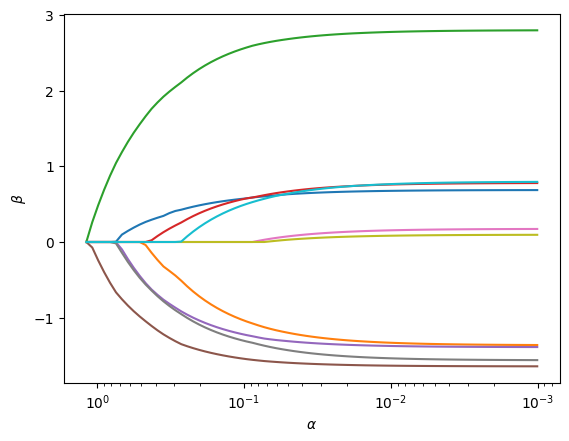
It also comes with a plot() method to visualize the path of coefficients:

fig, ax = res.plot()

Cross-Validation

It is also easy to cross-validate in the sortedl1 package. Since the estimator is scikit-learn compatible, we could use the functionality from scikit-learn directly, but sortedl1 also includes native cross-validation routines that are optimized for the SLOPE package.

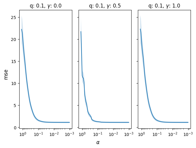
In the following example, we cross-validate across different levels of the gamma parameter, which fits the relaxed SLOPE model (a linear combination of SLOPE and ordinary least squares fit to the cluster structure from SLOPE).

cv_res = model.cv(x, y, q=[0.1], gamma=[0.0,0.5, 1.0])
fig, ax = cv_res.plot()

In this low-dimensional example, we see that there is, unsurprisingly, little benefit to regularization.