Chapter 2 Simple linear regression
2.1 playbill
First we load the data.
playbill <- read.csv(file.path("data", "playbill.csv"))Then we fit a linear model, \(Y=\beta_0 + \beta_1 + e\) and summarize it in Table 2.1.
pb_fit1 <- lm(CurrentWeek ~ LastWeek, data = playbill)
kable(summary(pb_fit1)$coef,
      booktabs = TRUE,
caption = "Coefficients our linear model.")| Estimate | Std. Error | t value | Pr(>|t|) | |
|---|---|---|---|---|
| (Intercept) | 6804.89 | 9929.32 | 0.69 | 0.5 |
| LastWeek | 0.98 | 0.01 | 68.07 | 0.0 |
a
The confidence intervals for \(\beta_1\) are given by
confint(pb_fit1)[2, ]## 2.5 % 97.5 %
## 0.95 1.01As per the question, 1 seems like a plausible value given that returns are likely to be similar from one week to another (although exactly 1 is incredibly unlikely).
b
We proceed to test the hypotheses \[ \begin{gather} H_0:\beta_0 = 10000 \\ H_1:\beta_0 \neq 10000 \end{gather} \]
by running
h_0 <- 10000
h_obs <- coef(pb_fit1)[[1]]
h_obs_se <- summary(pb_fit1)$coef[1, 2]

tobs <- (h_obs - h_0) / h_obs_se
(pobs <- 2 * pt(abs(tobs), nrow(playbill) - 2, lower.tail = FALSE))
## [1] 0.75which leads us to accept the null hypothesis, \(t(16) = -0.32\), \(p = 0.75\).
c
We make a prediction, including prediction interval, for a 400,000$ box office result in the previous week:
predict(pb_fit1, data.frame(LastWeek = 400000), interval = "prediction")## fit lwr upr
## 1 4e+05 359833 439442A prediction of 450,000$ is not feasible, given it is far outside our 95% prediction interval.
d
This seems like an okay rule given the almost-perfect correlation from one week to another; however, looking at the residuals we see that there are at least three values that are predicted badly (Figure 2.1)
par(mfrow = c(2, 2))
plot(pb_fit1)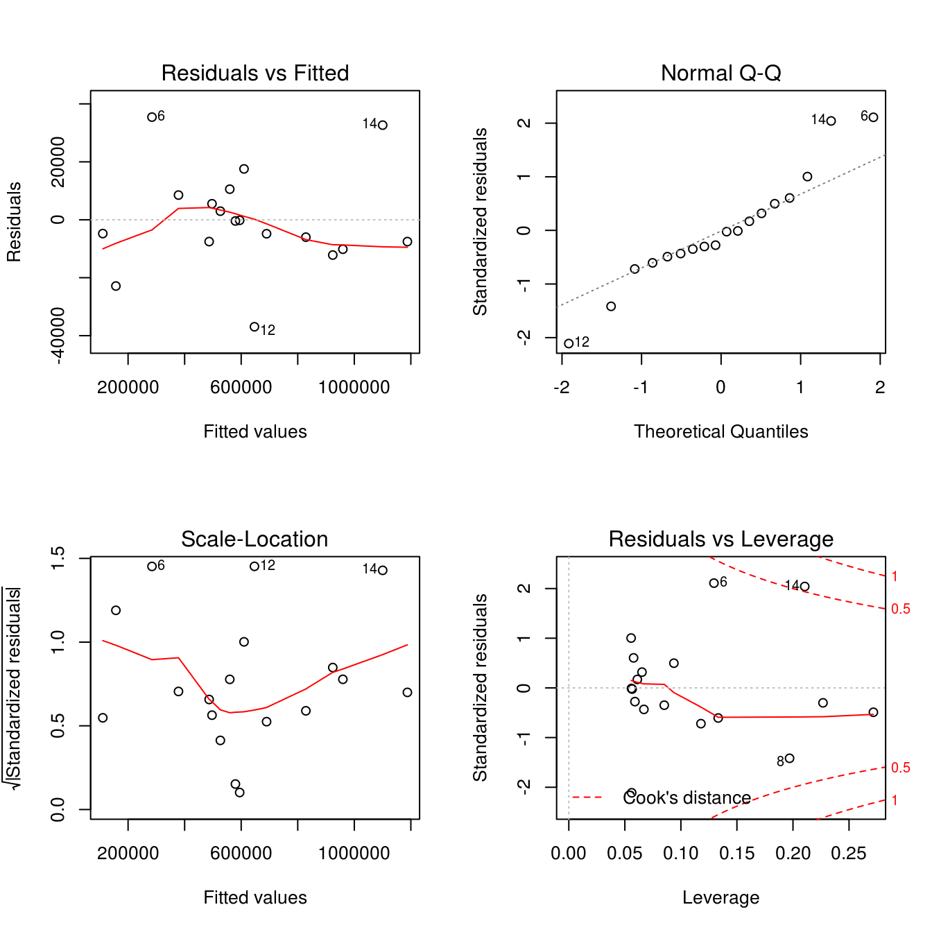
Figure 2.1: Residuals for our linear fit to the playbill data.
2.2 Indicators
indicators <- read.csv(file.path("data", "indicators.csv"))We begin by fitting our linear model to the data (Table 2.2).
ind_fit1 <- lm(PriceChange ~ LoanPaymentsOverdue, data = indicators)
kable(summary(ind_fit1)$coef,
      booktabs = TRUE,
caption = "Coefficients for our linear model to the indicators data set.")| Estimate | Std. Error | t value | Pr(>|t|) | |
|---|---|---|---|---|
| (Intercept) | 4.5 | 3.3 | 1.4 | 0.19 |
| LoanPaymentsOverdue | -2.2 | 0.9 | -2.5 | 0.02 |
a
The 95% confidence interval for the \(\beta_1\) estimate is, as before:
confint(ind_fit1)[2, ]## 2.5 % 97.5 %
## -4.16 -0.33There is reason to believe that there is a negative trend.
b
We now create a confidence interval for \(\text{E}[Y|X=4]\):
predict(ind_fit1, data.frame(LoanPaymentsOverdue = 4), interval = "confidence")## fit lwr upr
## 1 -4.5 -6.6 -2.30% is not a reasonable estimate for \(\text{E}[Y|X=4]\) since the 95% confidence limit is far below 0.
2.3 Invoices
a
We first find a 95% confidence level for \(\beta_0\) using the output printed in the book.
beta0 <- 0.6417099
beta0_se <- 0.122707
beta0_t <- 5.248
beta0_margin <- 1.96 * beta0_se
(beta0_95 <- c(beta0 - beta0_margin, beta0 + beta0_margin))
## [1] 0.40 0.88Thus, the confidence limit it 0.4, 0.88
b
We have the two-sided hypotheses \[\begin{gathered} H_0: \beta_1 = 0.01\\ H_1: \beta_1 \neq 0.01. \end{gathered}\]
beta <- 0.01
beta_obs_se <- 0.0008184
beta_obs <- 0.0112916
tval <- (beta - beta_obs) / beta_obs_se
(pobs <- 2 * pt(abs(tval), 30 - 1, lower.tail = FALSE))
## [1] 0.13We fail to reject the null hypothesis, \(t(29) = -1.58\), \(p=0.13\). We cannot say that the true average processing time is significantly different from 0.01 hours.
c
From the exercise description we have the expected value \[ \text{Time} = 0.6417099+\text{Invoices}\times 0.0112916 \] for the series. Next, we’ll predict the processing time for 130 invoices using the output given in the exercise.
beta0 <- 0.6417099
beta1 <- 0.0112916
rse <- 0.3298
n <- 30
df <- n - 2
rss <- rse^2 * df
mse <- rss / n

time <- beta0 + beta1 * 130
err <- qt(0.975, 28) * sqrt(mse) * sqrt(1 + 1 / n) # since x0 = xbar
upr <- time + err
lwr <- time - err
Which results in a point estimate of 2.11, 95% CI: \([1.45, 2.77]\).
2.4 Straight-line regression through the origin
a
We shall show that \[ \hat{\beta} = \frac{\sum_{i=1}^n x_iy_i}{\sum_{i=1}^n x_i^2}. \] We have \[ Y_i = \beta x_i + e_i, \] which has the least-squares solution of \[ \text{RSS} = \sum_{i=1}^n (y_i-\hat{y}_i)^2 = \sum_{i=1}^n(y_i-\hat{\beta}x_i)^2 \] that is solved by setting its partial derivative with respect to \(\beta\) to 0, like so: \begin{align} \frac{\partial}{\partial \beta}\text{RSS} = -2 \sum_{i=1}^nx_i(y_i - \hat{\beta}x_i) & = 0 \iff \\ \sum_{i=1}^nx_iy_i - \hat{\beta} \sum_{i=1}^n x_i^2 & = 0 \iff \\ \hat{\beta} & = \frac{\sum_{i=1}^n x_i y_i}{\sum_{i=1}^nx_i} \tag*{$\square$}. \end{align}b
- \[ E(\hat{\beta} | X) = E\left( \frac{\sum_{i=1}^n x_i y_i}{\sum_{i=1}^n x_i^2} \right) = \frac{\sum_{i=1}^n x_i E(y_i)}{\sum_{i=1}^n x_i^2 } = \beta \frac{\sum_{i=1}^nx_i^2}{\sum_{i=1}^n x_i^2} = \beta \tag*{$\square$} \]
- \[ \text{Var}(\hat{\beta}|X) = \text{Var} \left( \frac{\sum_{i=1}^nx_iy_i}{\sum_{i=1}^n x_i^2}\right) = \frac{\sum_{i=1}^n x_i^2\sigma^2}{\left( \sum_{i=1}^n x_i^2 \right)^2} = \frac{\sigma^2}{\sum_{i=1}^n x_i^2} \tag*{$\square$} \]
- Follows from (1) and (2).
2.5 Multiple choices
- is correct. SSreg is larger in model 1 because the model explains more of the variance, whilst RSS is smaller since there is less variance left unexplained.
2.6 SST = SSreg + RSS
a
\[ y_i - \hat{y}_i = (y_i - \bar{y}) - (\hat{y}_i - \bar{y}) = (y_i - \bar{y}) - (\hat{\beta}x_i - \hat{\beta}\bar{x}) = (y_i - \bar{y}) - \hat{\beta}(x_i - \bar{x}) \tag*{$\square$} \]
b
\[ \hat{y}_i - \bar{y} = \hat{\beta}x_i - \hat{\beta}\bar{x} = \hat{\beta}(x_i - \bar{x}) \tag*{$\square$} \]
c
\[ \begin{gathered} \sum_{i=1}^n (y_i-\hat{y}_i)(\hat{y}_i - \bar{y}) = \sum_{i=1}^n (y_i - \hat{\beta_0} - \hat{\beta_1}x_i)\hat{\beta}_1(x_i - \bar{x}) = \\ \hat{\beta}_1 \left( \sum_{i=1}^n y_i(x_i \bar{x}) - \hat{\beta}_0 \sum_{i=1}^n x_i - \bar{x} - \hat{\beta}_1 \sum_{i=1}^n x_i(x_i - \bar{x}) \right) = \\ \hat{\beta_1}(\text{SXY} - 0 - \hat{\beta_1} \text{SXX}) = \\ \hat{\beta_1}(SXY - SXY) = 0 \qquad \square \end{gathered} \]
2.7 Confidence intervals
It is possible since the confidence interval is designed to contain the population regression line 0.95 of the time and not 95% of the observations – which is what the prediction interval is meant to do.