Easy

Our first task is to fit a L1-regularized linear model to the spam data set from ElemStatLearn and analyze the results in terms of the selected features as well as test error and AUC. We will also compare our model to a naive model that predicts the most frequent class.

We begin by loading our libraries.

library(gsoc18saga)
library(glmnet)
library(ElemStatLearn)

We will use the ElemStatLearn::spam dataset to try to classify email as either spam or regular email. We load the data and set up balanced train and test partitions using the caret package.

# extract the necessary data
x <- as.matrix(spam[, -ncol(spam)])
y <- spam$spam
n <- nrow(x)

# create train and test sets
train_id <- caret::createDataPartition(y, p = 0.75)[[1L]]
train_x <- x[train_id, ]
train_y <- y[train_id]
test_x <- x[-train_id, ]
test_y <- y[-train_id]

# train the model
set.seed(1)
fit <- glmnet::cv.glmnet(train_x, train_y, family = "binomial")

The model’s chosen features are

names(coef(fit)[coef(fit)[, 1] > 0, ])
#>  [1] "A.3"  "A.4"  "A.5"  "A.6"  "A.7"  "A.8"  "A.9"  "A.10" "A.15" "A.16"
#> [11] "A.17" "A.18" "A.19" "A.20" "A.21" "A.22" "A.23" "A.24" "A.36" "A.52"
#> [21] "A.53" "A.54" "A.56" "A.57"

Next we’ll examine the performance of the model using Receiver Operating Characteristics (ROC), Area Under the Curve (AUC), and test error. We’ll compare the model against a naive classification scheme wherein we predict each observation (email) to be the most prevalent category of the training set, namely. email.

library(pROC)

roc_glmnet <- roc(test_y,
                  as.vector(predict(fit, test_x, type = "response")),
                  ci = TRUE)
roc_naive <- roc(test_y, rep(1, length(test_y)), ci = TRUE)

plot(roc_glmnet, print.auc = TRUE)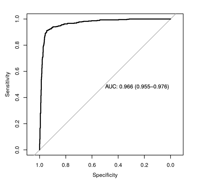

Receiver operating characteristic curves for the lasso model.

The 95% confidence level for the AUC value for our lasso model is \([0.955414, 0.9760234]\). We can compare the glmnet model to the naive model using DeLong’s test

roc.test(roc_glmnet, roc_naive)
#> 
#>  DeLong's test for two correlated ROC curves
#> 
#> data:  roc_glmnet and roc_naive
#> Z = 88.58, p-value < 2.2e-16
#> alternative hypothesis: true difference in AUC is not equal to 0
#> sample estimates:
#> AUC of roc1 AUC of roc2 
#>   0.9657187   0.5000000

which unsurprisingly shows that the glmnet model is significantly better. Looking at the accuracy of the model, the naive model has an accuracy of 0.606087 whilst the lasso model manages an accuracy of 0.9313043.

Medium

In this part we are going to compare the performance of glmnet with that of bigoptim for L2-regularized model fits. For this purpose, we are going to use the gsoc18saga::covertype data set and and see how timings differ depending on the numbers of columns and rows we use from the data. We will also study objective function values in the same fashion.

The results for these simulations have been precomputed through code that is available at https://github.com/jolars/gsoc18saga/blob/master/data-raw/medium.R. The dataset is made part of this package and available as gsoc18saga::data_medium.

Looking at the results from the simulation, we note that glmnet() and sag_fit() (bigoptim) perform on par with one another when either the rows or columns are relatively few. As we add more observations (rows) and covariates (columns), however, the SAG algorithm from bigoptim outperforms glmnet() in speed.

gradpal <- colorRampPalette(RColorBrewer::brewer.pal(11, "RdBu"))(100)

library(tidyr)
library(dplyr)

data_medium_diff <- data_medium %>%
  gather("var", "value", time, loss) %>%
  spread(package, value) %>%
  mutate(diff = glmnet - sag) %>%
  select(-glmnet, -sag) %>%
  spread(var, diff)

z <- max(abs(data_medium_diff$time))

lattice::levelplot(
  time ~ cols*rows, 
  data = data_medium_diff,
  asp = 1,
  at = seq(-z, z, length.out = 20),
  col.regions = gradpal,
  main = "Speed (glmnet - bigoptim)"
)

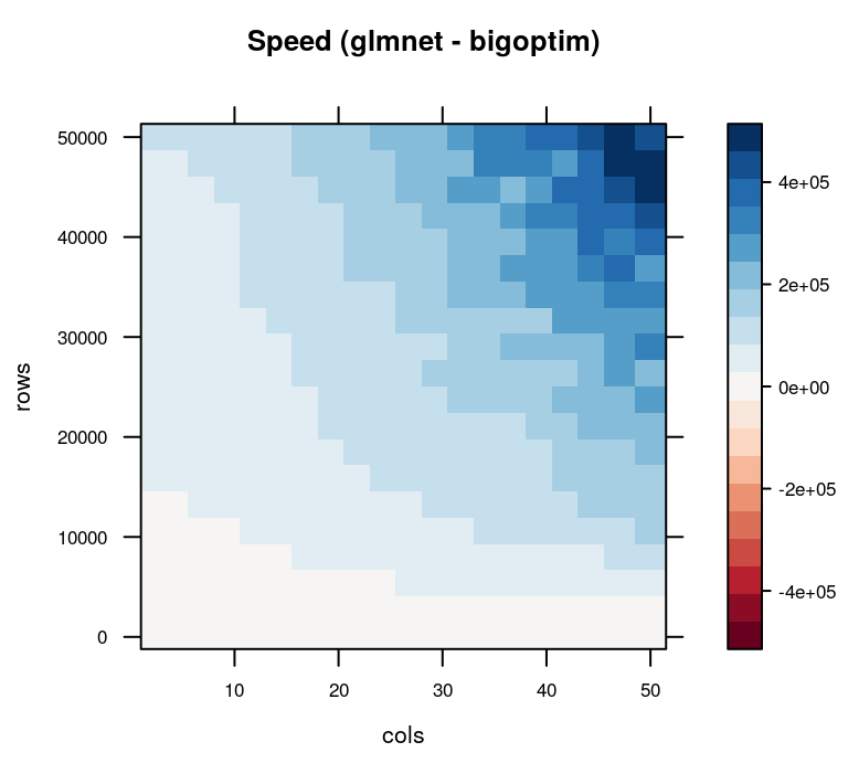
Speed in microseconds of glmnet and bigoptim runs. Positive values (blue) favor bigoptim.

In terms of loss, however, we see that bigoptim suffers when there are many features in the model, particularly when the number of observations are relatively low.

z <- max(abs(data_medium_diff$loss))
lattice::levelplot(
  loss ~ cols*rows,
  data = data_medium_diff,
  asp = 1,
  at = seq(-z, z, length.out = 20),
  col.regions = gradpal,
  main = "Loss (glmnet - bigoptim)"
)

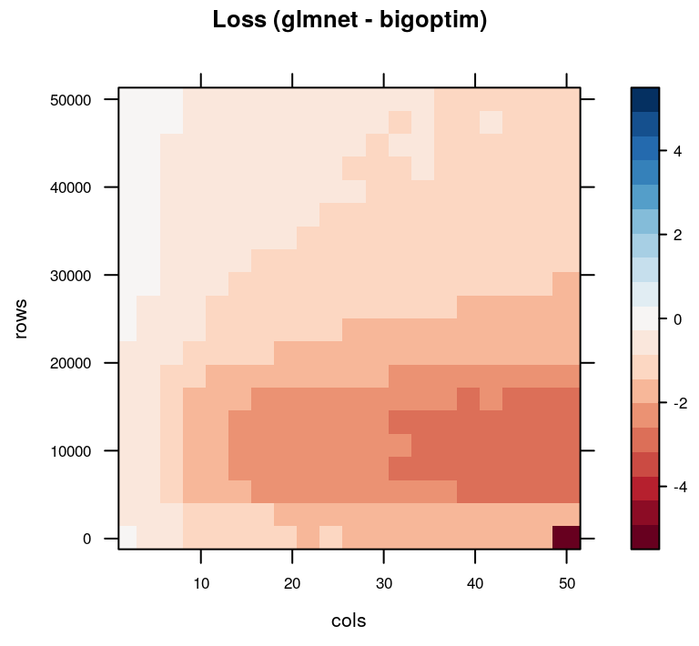
Difference in objective function loss for glmnet and bigoptim. Negative (red) values favor glmnet.

Medium-hard

This section is similar to the previous one but relates to L1-regularization, rather than L2-regularization and instead compares glmnet with the logistic regression fitter of the python scikit-learn module. In particular, we will look at the SAGA algorithm. This time around, we will look at six different datasets:

Name	Observations	Features
icjnn1	49,990	22
a9a	32,561	123
phishing	11,055	68
mushroooms	8,124	112
covtype	581,012	54
skin_nonskin	245,057	3

All of these have been collected from the libsvm binary dataset collection.

The R package reticulate is used to interface with python in the data simulations, which, are featured at https://github.com/jolars/gsoc18saga/blob/master/data-raw/medium-hard.R. The dataset is made part of this package and available as gsoc18saga::data_mediumhard.

To put the two packages on equal footing, we now instead use the python-based implementation of glmnet to circumvent the possible overhead that calling python from R might introduce. For each dataset in our comparison, we iterate across a range of tolerance values (stopping criteria) for the optimizers in the two algorithms and collect the objective loss for each algorithm as well as the runtime at which they terminate.

library(latticeExtra)
lattice::xyplot(loss ~ time | dataset,
                data_mediumhard,
                xlab = "Time (s)",
                ylab = "Objective loss",
                groups = package,
                scales = list(relation = "free"),
                auto.key = list(lines = TRUE, points = TRUE)) +
  glayer(panel.smoother(..., span = 0.5))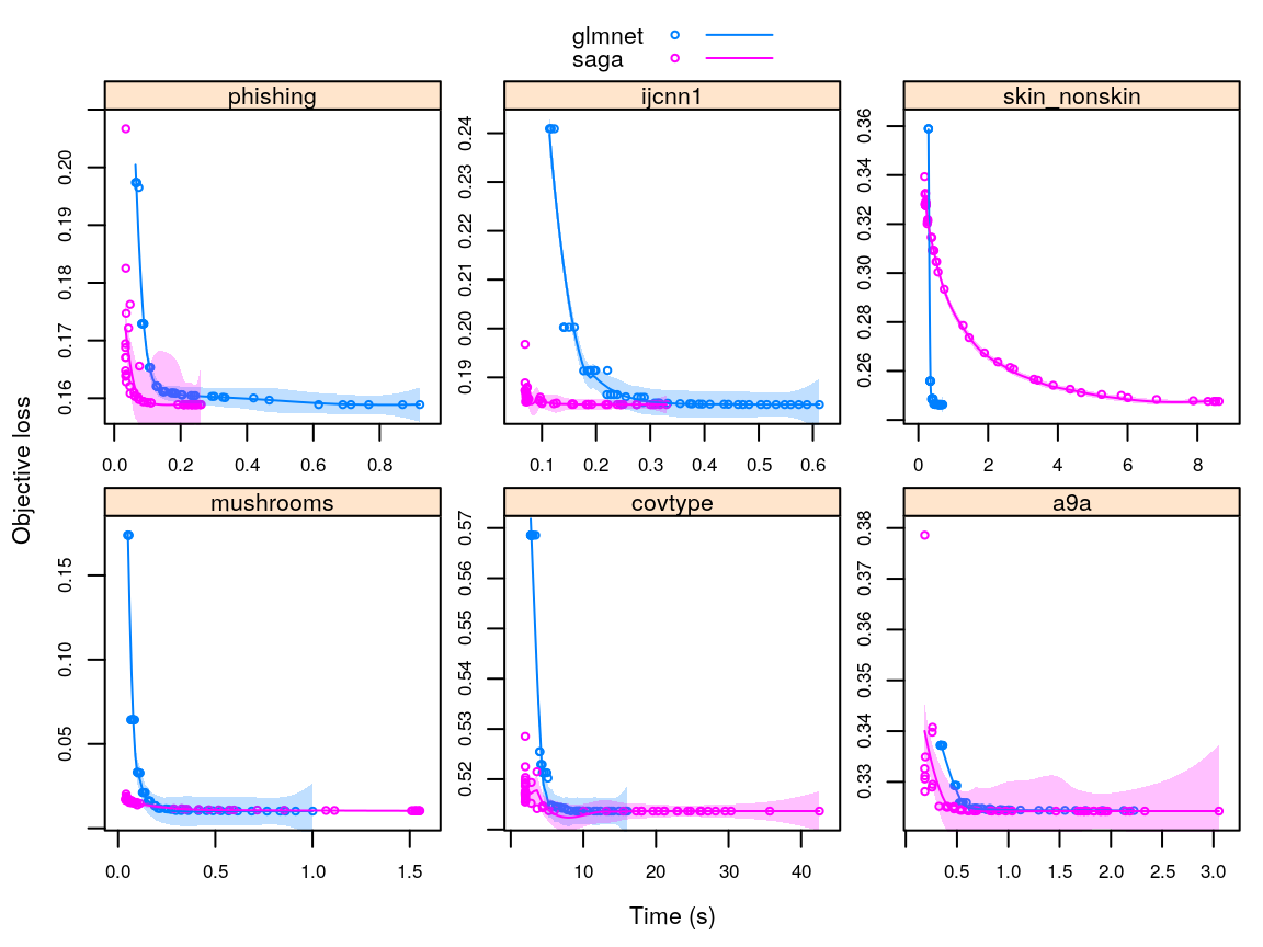

Objective loss and runtimes for the glmnet and SAGA implementations. The lines are Loess fits.

For all but the gsoc18saga::ijcnn1 dataset, the SAGA algorithm converges faster towards the minimum than glmnet, suggesting that there likely is benefit to be gained from porting the SAGA algorithm to R.

Hard

The solution to the last test is presented in the package that this vignette is part of. I have written the functions objective_r():

objective_r <- function(beta0, beta, x, y, lambda, alpha = 0) {
  n <- length(y)
  # binomial loglikelihood
  z <- beta0 + crossprod(x, beta)
  loglik <- sum(y*z - log(1 + exp(z)))

  # compute penalty
  penalty <- 0.5*(1 - alpha)*sum(beta^2) + alpha*sum(abs(beta))
  -loglik/n + lambda*penalty
}

and objective_cpp():

#include <RcppArmadillo.h>

// [[Rcpp::export]]
double objective_cpp(double beta0,
                     arma::vec beta,
                     arma::mat x,
                     arma::uvec y,
                     double lambda,
                     double alpha = 0) {
  int n = y.n_elem;
  arma::mat z = beta0 + x.t()*beta;
  double loglik = arma::accu(y%z - arma::log(1 + arma::exp(z)));
  double penalty = 0.5*(1 - alpha)*arma::accu(arma::square(beta)) +
    alpha*arma::accu(arma::abs(beta));
  return -loglik/n + lambda*penalty;
}

The concurrence of the two functions is examplified through the following lines, which have been added as a unit test to the package, the result of which you can view here, as required by the GSoC test.

# fit a L1-regularized logistic regression
x <- matrix(rnorm(100*20), 100, 20)
y <- sample(1:2, 100, replace = TRUE)
alpha <- 1
fit <- glmnet::cv.glmnet(x, y, family = "binomial", alpha = alpha)

# collect parameters
lambda <- fit$lambda.1se
beta0 <- coef(fit, lambda)[1]
beta <- coef(fit, lambda)[-1]

# compute objective function values
obj_r <- objective_r(beta0, beta, t(x), y, lambda, alpha = alpha)
obj_cpp <- objective_cpp(beta0, beta, t(x), y, lambda, alpha = alpha)

# check for equality
all.equal(obj_r, obj_cpp)
#> [1] TRUE