Background
The functions in this package solves problems of the type \[ \mathrm{minimize}\left\{f(\beta) + J(\beta; \sigma,\lambda) \right\}, \] where the second part of the objective is the sorted L1-norm, or equivalently the OWL norm, defined as \[ J(\beta; \sigma,\lambda) = \sigma \sum_{j=1}^p \lambda_j \lvert \beta \rvert_{(j)}, \] where \(\sigma \in \mathbb{R}_{+}\), \(\lambda \in \mathbb{R}_+^p\) and \((j)\) represents an rank of the magnitudes of \(\beta\) in descending order. \(\lambda\) controls the shape of the penalty sequence, which needs to be non-increasing, and \(\sigma\) controls the scale of that sequence.
Solving this problem is called SLOPE (Sorted L-One Penalized Estimation) (Bogdan et al. 2015) or OWL (Ordered Weighted L1) regression (Zeng and Figueiredo 2014)—hence the name of the package.
In this problem, \(f(\beta)\) is a smooth and convex objective, which for this package so far includes four models from the family of generalized linear models:
- Gaussian regression,
- binomial regression,
- multinomial regression, and
- poisson regression.
SLOPE is an extension of the lasso (Tibshirani 1996) and has the ability to lead to sparse solutions given a sufficiently strong regularization. It is also easy to see that SLOPE reduces to the lasso if all elements of the \(\lambda\) vector are equal.
The lasso, however, has difficulties with correlated predictors (Jia and Yu 2010) but this is not the case with SLOPE, which handles this issue by clustering predictors to the same magnitude. This effect is related to the consecutive differences of the \(\lambda\) vector: the larger the steps, the more clustering behavior SLOPE exhibits.
An example
In the following example, we will use the heart data set, for which the response is a cardiac event. (The package contains several data sets to exemplify modeling. Please see the examples in owl().) The main function of the package is owl(), which, more or less, serves as an interface for code written in C++. There are many arguments in the function and most of them relate to either the construction of the regularization path or the penalty (\(\lambda\)) sequence used. Here we will use the option lambda = "bh", which used the BH method detailed in Bogdan et al. (2015) to select the sequence. (Note that it is also possible to manually insert a sequence.)
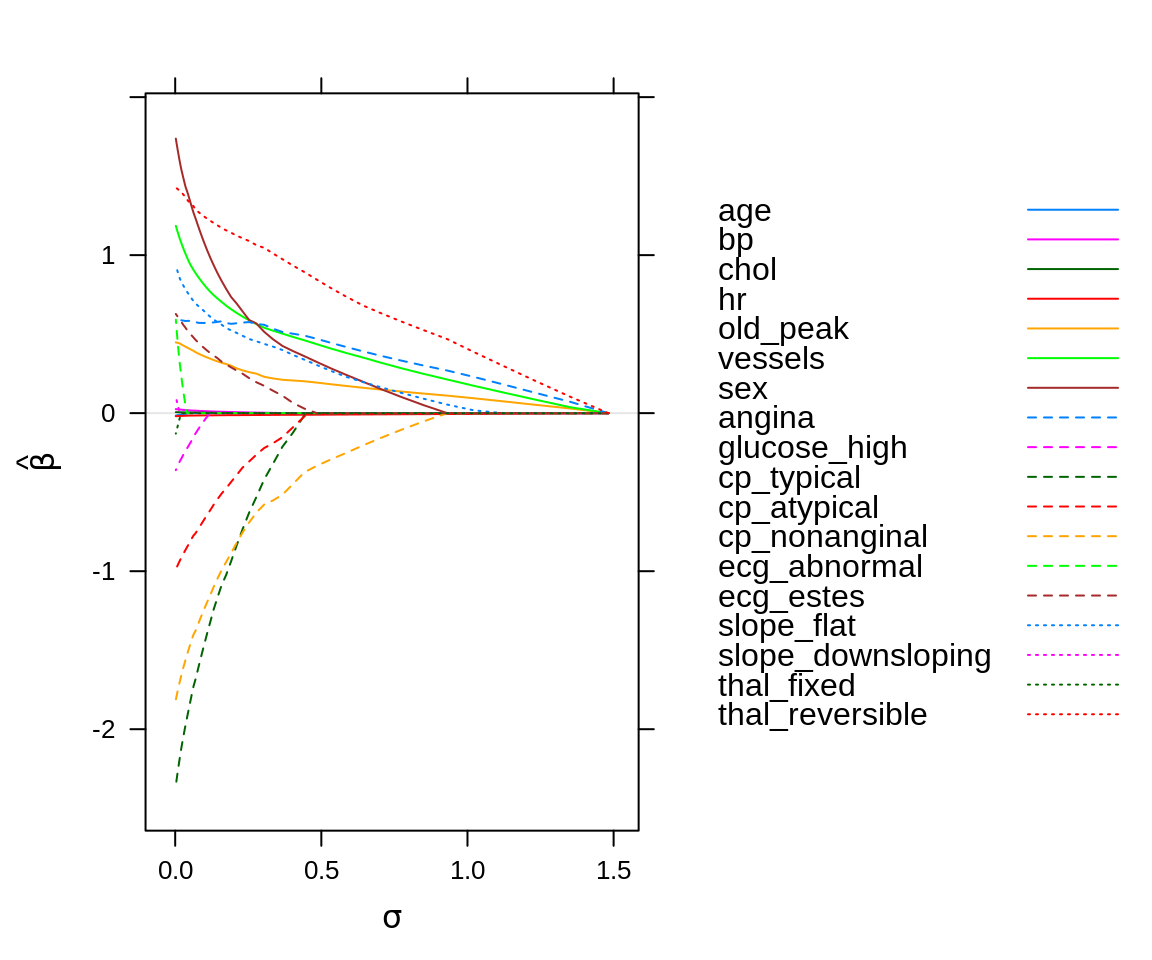
The default print method gives a summary of the regularization path but it is usually more informative to study a plot of the path.

Regularization path for a binomial regression model fit to the heart data set.
Cross-validation
To determine the strength of regularization, it is almost always necessary to tune the \(\lambda\) sequence using resampling. This package features two methods for this: a specification for use with the caret package via the function caretSlopeOwl() or trainOwl(). While former facilitate easier comparison of SLOPE against other methods as well as a multitude of options for resampling and measuring performance, it does not allow for sparse predictor matrices. We will give an example of trainOwl() here.
set.seed(924)

x <- bodyfat$x
y <- bodyfat$y

tune <- trainOwl(x,
                 y,
                 q = c(0.1, 0.2),
                 number = 10,
                 repeats = 3)
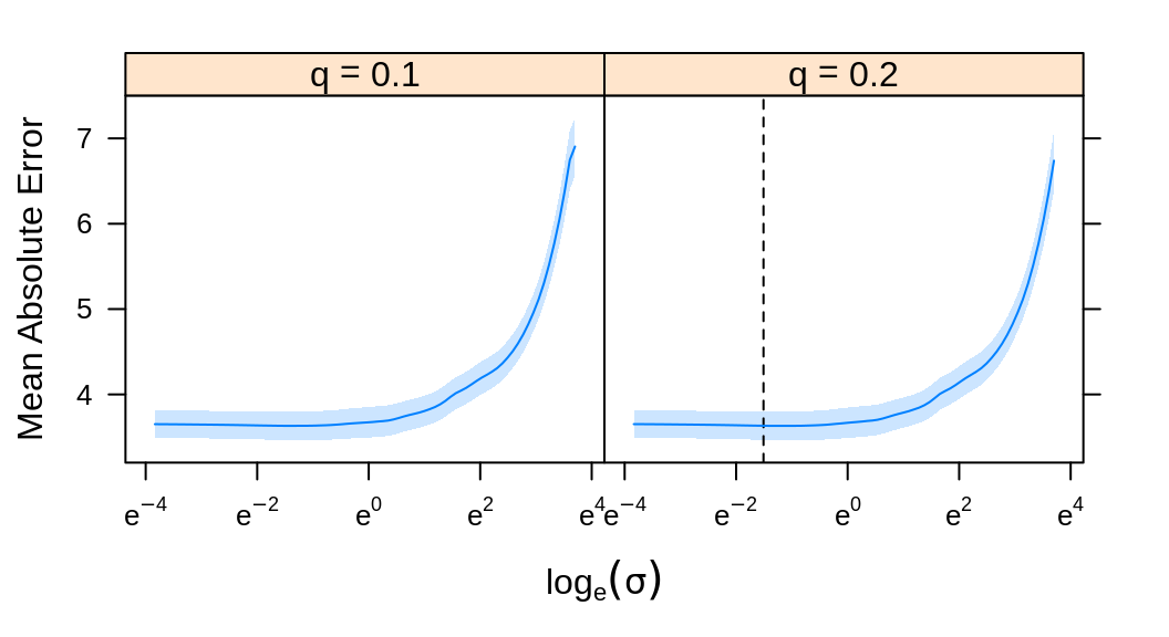
As before, the plot method offers the best summary.

Model tuning results from Gaussian SLOPE on the bodyfat dataset.
Printing the resulting object will display the optimum values
False discovery rate
Under assumptions of orthonormality, SLOPE has been shown to control false discovery rate (FDR) of non-zero coefficients (feature weights) in the model (Bogdan et al. 2015). It is in many ways analogous to the Benjamini–Hochberg procedure for multiple comparisons.
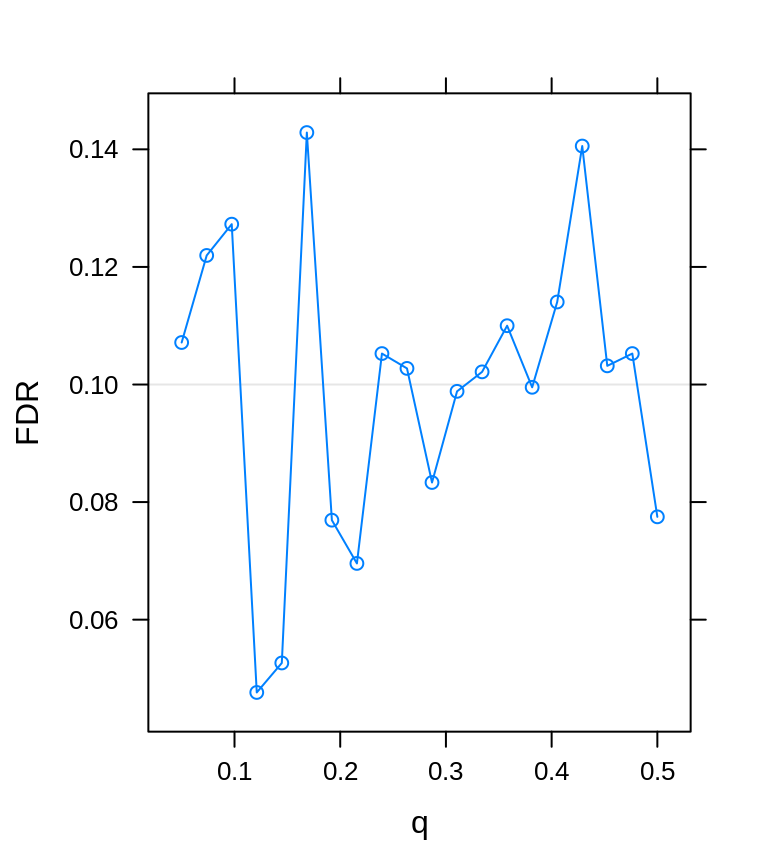
Let’s set up a simple experiment to see how SLOPE controls the FDR. We randomly generate data sets with various proportions of true signals. Under this gaussian design with independently and identically distributed columns in \(X\), SLOPE should asymptotically control FDR at the level given by the shape parameter \(q\), which we set to 0.1 in this example.
# proportion of real signals
q <- seq(0.05, 0.5, length.out = 20)
fdr <- double(length(q))
set.seed(1)

for (i in seq_along(q)) {
  n <- 1000
  p <- n/2
  sigma <- 1
  problem <- owl:::randomProblem(n, p, q = q[i], sigma = sigma)

  x <- problem$x
  y <- problem$y
  signals <- problem$nonzero

  fit <- owl(x,
             y,
             lambda = "gaussian",
             q = 0.1,
             sigma = sigma)

  selected_owl <- which(fit$nonzeros)
  V <- length(setdiff(selected_owl, signals))
  R <- length(selected_owl)
  fdr[i] <- V/R
}

library(lattice)
xyplot(fdr ~ q, type = "b", ylab = "FDR",
       panel = function(...) {
         panel.refline(h = 0.1)
         panel.xyplot(...)
       })
Control of false discovery rate using SLOPE.
SLOPE seems to control FDR at roughly the specified level.
References
Bogdan, Małgorzata, Ewout van den Berg, Chiara Sabatti, Weijie Su, and Emmanuel J. Candès. 2015. “SLOPE – Adaptive Variable Selection via Convex Optimization.” The Annals of Applied Statistics 9 (3): 1103–40. https://doi.org/10/gfgwzt.
Jia, J., and B. Yu. 2010. “On Model Selection Consistency of the Elastic Net When P \(>>\) N.” Statistica Sinica 20 (2): 595–611.
Tibshirani, Robert. 1996. “Regression Shrinkage and Selection via the Lasso.” Journal of the Royal Statistical Society. Series B (Methodological) 58 (1): 267–88.
Zeng, Xiangrong, and Mário A. T. Figueiredo. 2014. “The Atomic Norm Formulation of OSCAR Regularization with Application to the Frank-Wolfe Algorithm.” In 2014 22nd European Signal Processing Conference (EUSIPCO), 780–84.