2 Fundamental concepts

2.1 Basic properties of expected value and covariance

a

\begin{align} \text{Cov}[X,Y] & = \text{Corr}[X,Y]\sqrt{Var[X]Var[Y]}\\ & = 0.25 \sqrt{9 \times 4} = 1.5 \\ \text{Var}[X,Y] & = Var[X]+Var[Y]+2Cov[X,Y]\\ & = 9 + 4 + 2 \times 3 = 16\\ \end{align}

b

\[\text{Cov}[X, X+Y] = \text{Cov}[X,X] + \text{Cov}[X,Y] = \text{Var}[X] + \text{Cov}[X,Y] = 9 + 1.5 = 10.5\]

c

\begin{align} \text{Corr}[X+Y, X-Y] = & \text{Corr}[X,X] + \text{Corr}[X,-Y] + \text{Corr}[Y,X] + \text{Corr}[Y,-Y] \\ = & \text{Corr}[Y,X] + \text{Corr}[Y,-Y] \\ = & 1 - 0.25 + 0.25 -1 \\ = & 0 \\ \end{align}

2.2 Dependence and covariance

\begin{gather*} \text{Cov}[X+Y,X-Y] = \text{Cov}[X,X] + \text{Cov}[X,-Y] + \text{Cov}[Y,X] + \text{Cov}[Y, -Y] = \\ Var[X] - Cov[X,Y] + Cov[X,Y] - Var[Y] = 0 \end{gather*}

since \(Var[X] = Var[Y]\).

2.3 Strict and weak stationarity

a

We have that \begin{gather*} P(Y_{t_1}, Y_{t_2}, \dots, Y_{t_n}) = \\ P(X_1, X_2, \dots, X_n) = \\ P(Y_{t_1 - k}, Y_{t_2 - k}, \dots, Y_{t_n - k}), \end{gather*}

which satisfies our requirement for strict stationarity.

b

The autocovariance is given by \begin{gather*} \gamma_{t,s}=\text{Cov}[Y_t, Y_s] = \text{Cov}[X,X] = \text{Var}[X] = \sigma^2. \end{gather*}

c

library(lattice)
tstest <- ts(runif(100))

lattice::xyplot(tstest,
                panel = function(x, y, ...) {
                  panel.abline(h = mean(y), lty = 2)
                  panel.xyplot(x, y, ...)
                })

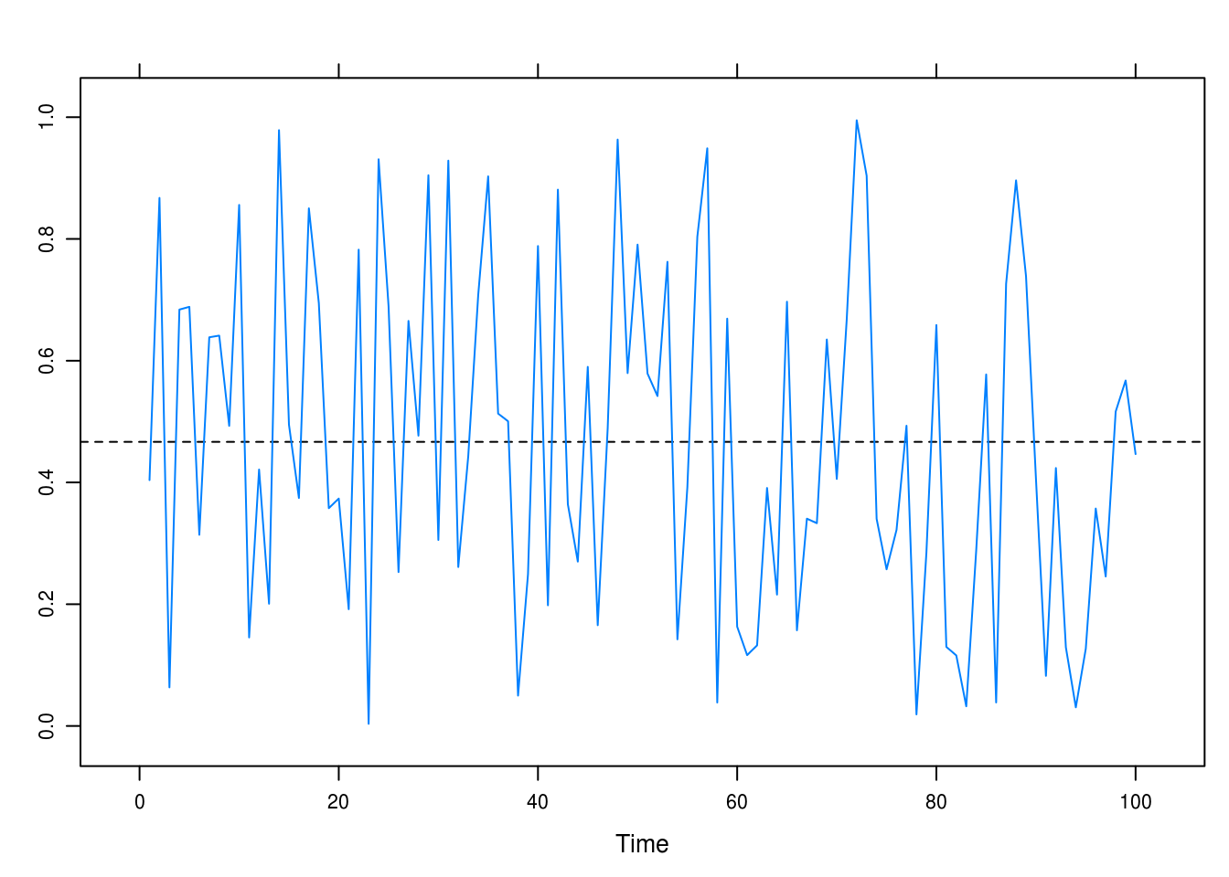
Figure 2.1: A white noise time series: no drift, independence between observations.

2.4 Zero-mean white noise

a

\begin{gather*} E[Y_t] = E[e_t+\theta e_{t-1}] = E[e_t] + \theta E[e_{t-1}] = 0 + 0 = 0\\ V[Y_t] = V[e_t + \theta e_{t-1}] = V[e_t] + \theta^2 V[e_{t-1}] = \sigma_e^2 + \theta^2 \sigma_e^2 = \sigma_2^2(1 + \theta^2)\\ \end{gather*}

For \(k = 1\) we have

\begin{gather*} C[e_t + \theta e_{t-1}, e_{t-1} + \theta e_{t-2}] = \\ C[e_t,e_{t-1}] + C[e_t, \theta e_{t-2}] + C[\theta e_{t-1}, e_{t-1}] + C[\theta e_{t-1}, \theta e_{t-2}] = \\ 0 + 0 + \theta V[e_{t-1}] + 0 = \theta \sigma_e^2,\\ \text{Corr}[Y_t, Y_{t-k}] = \frac{\theta \sigma_e^2}{\sqrt{(\sigma_e^2(1+\theta^2))^2}} = \frac{\theta }{1+\theta^2} \end{gather*}

and for \(k = 0\) we get

\begin{gather*} \text{Corr}[Y_t, Y_{t-k}] = \text{Corr}[Y_t, Y_t] = 1 \end{gather*}

and, finally, for \(k > 0\):

\begin{gather*} C[e_t + \theta e_{t-1}, e_{t-k} + \theta e_{t-k-1}] = \\ C[e_t, e_{t-k}] + C[e_t, e_{t-1-k}] + C[\theta e_{t-1}, e_{t-k}] + C[\theta e_{t-1}, \theta e_{t-1-k}] = 0 \end{gather*}

given that all terms are independent. Taken together, we have that

\begin{gather*} \text{Corr}[Y_t, Y_{t-k}] = \begin{cases} 1 & \quad \text{for } k = 0\\ \frac{\theta}{1 + \theta^2} & \quad \text{for } k = 1\\ 0 & \quad \text{for } k > 1 \end{cases}. \end{gather*}

And, as required,

\begin{gather*} \text{Corr}[Y_t, Y_{t-k}] = \begin{cases} \frac{3}{1+3^2} = \frac{3}{10} & \quad \text{if } \theta = 3\\ \frac{1/3}{1 + (1/3)^2} = \frac{1}{10/3} = \frac{3}{10} & \quad \text{if } \theta = 1/3 \end{cases}. \end{gather*}

b

No, probably not. Given that \(\rho\) is standardized, we will not be able to detect any difference in the variance regardless of the values of k.

2.5 Zero-mean stationary series

a

\[\mu_t = E[Y_t] = E[5 + 2t + X_t] = 5 + 2E[t] + E[X_t] = 5 + 2t + 0 = 2t + 5\]

b

\[ \gamma_k = \text{Corr}[5+2t+X_t, 5+2(t-k)+X_{t-k}] = \text{Corr}[X_t, X_{t-k}]\]

c

No, the mean function (\(\mu_t\)) is constant and the aurocovariance (\(\gamma_{t,t-k}\)) free from \(t\).

2.6 Stationary time series

a

\begin{gather*}\text{Cov}[a + X_t, b + X_{t-k}] =\text{Cov}[X_t, X_{t-k}],\end{gather*}

which is free from \(t\) for all \(k\) because \(X_t\) is stationary.

b

\begin{gather*} \mu_t = E[Y_t] = \begin{cases} E[X_t] & \quad \text{for odd } t\\ 3 + E[X_t] & \quad \text{for even } t\\ \end{cases}. \end{gather*}

Since \(\mu_t\) varies depending on \(t\), \(Y_t\) is not stationary.

2.7 First and second-order difference series

a

\begin{gather*}\mu_t = E[W_t] = E[Y_t - Y_{t-1}] = E[Y_t] - E[Y_{t-1}] = 0\end{gather*}

because \(Y_t\) is stationary.

\begin{gather*} \text{Cov}[W_t] = \text{Cov}[Y_t - Y_{t-1}, Y_{t-k} - Y_{t-1-k}] = \\ \text{Cov}[Y_t, Y_{t-k}] + \text{Cov}[Y_t, Y_{t-1-k}] + \text{Cov}[-Y_{t-k}, Y_{t-k}] + \text{Cov}[-Y_{t-k}, -Y_{t-1-k}]=\\ \gamma_k-\gamma_{k+1}-\gamma_{k-1}+\gamma_{k} = 2 \gamma_k - \gamma_{k+1} - \gamma_{k-1}. \quad \square \end{gather*}

b

In (a), we discovered that the difference between two stationary processes, \(\triangledown Y_t\) itself was stationary. It follows that the difference between two of these differences, \(\triangledown^2Y_t\) is also stationary.

2.8 Generalized difference series

\begin{align} E[W_t] & = c_1E[Y_t]+c_2E[Y_t] + \dots + c_n E[Y_t]\\ & = E[Y_t](c_1 + c_2 + \dots + c_n), \end{align}

and thus the expected value is constant. Moreover,

\begin{align} \text{Cov}[W_t] & = \text{Cov}[c_1 Y_t + c_2 Y_{t-1} + \dots + c_n Y_{t-k}, c_1 Y_{t-k} + c_2 Y_{t-k-1} + \dots + c_n Y_{t-k-n}] \\ & = \sum_{i=0}^n \sum_{j=0}^n c_i c_j \text{Cov}[Y_{t-j}Y_{t-i-k}] \\ & = \sum_{i=0}^n \sum_{j=0}^n c_i c_j \gamma_{j-k-i}, \end{align}

which is free of \(t\); consequently, \(W_t\) is stationary.

2.9 Zero-mean stationary difference series

a

\begin{gather*} E[Y_t] = \beta_0 + \beta_1 t + E[X_t] = \beta_0 + \beta_1 t + \mu_{t_x}, \end{gather*}

which is not free of \(t\) and hence not stationary.

\begin{gather*} \text{Cov}[Y_t] = \text{Cov}[X_t, X_t-1] = \gamma_{t-1} \end{gather*} \begin{gather*} E[W_t] = E[Y_t - Y_{t-1}] = E[\beta_0 + \beta_1 t + X_t - (\beta_0 + \beta_1(t-1) + X_{t-1})] =\\ \beta_0 + \beta_1 t - \beta_0 - \beta_1 t + \beta_1 = \beta_1, \end{gather*}

is free of \(t\) and, furthermore, we have

\begin{gather*} \text{Cov}[W_t] = \text{Cov}[\beta_0 + \beta_1 t + X_t, \beta_0 + \beta_1 (t-1) + X_{t-1}] =\\ \text{Cov}[X_t, X_{t-1}] = \gamma_k, \end{gather*}

which is also free of \(t\), thereby proving that \(W_t\) is stationary.

b

\begin{gather*} E[Y_t] = E[\mu_t + X_t] = \mu_t + \mu_t = 0 + 0 = 0, \quad \text{and}\\ \text{Cov}[Y_t] = \text{Cov}[\mu_t + X_t, \mu_{t-k} + X_{t-k}] = \text{Cov}[X_t, X_{t-k}] = \gamma_k \end{gather*} \begin{gather*} \triangledown^m Y_t = \triangledown(\triangledown^{m−1}Y_t) \end{gather*}

Currently unsolved.

2.10 Zero-mean, unit-variance process

a

\begin{gather*} \mu_t = E[Y_t] = E[\mu_t + \sigma_t X_t] = \mu_t + \sigma_t E[X_t] = \mu_t + \sigma_t \times 0 = \mu_t\\ \gamma_{t,t-k} = \text{Cov}[Y_t] = \text{Cov}[\mu_t + \sigma_t X_t, \mu_{t-k} + \sigma_{t-k} X_{t-k}] = \sigma_t \sigma_{t-k} \text{Cov}[X_t, X_{t-k}] = \sigma_t \sigma_{t-k} \rho_k \end{gather*}

b

First, we have \begin{gather*} \text{Var}[Y_t] = \text{Var}[\mu_t + \sigma_t X_t] = 0 + \sigma_t^2 \text{Var}[X_t] = \sigma_t^2 \times 1 = \sigma_t^2 \end{gather*}

since \(\{X_t\}\) has unit-variance. Futhermore,

\begin{gather*} \text{Corr}[Y_t, Y_{t-k}] = \frac{\sigma_t \sigma_{t-k} \rho_k}{\sqrt{\text{Var}[Y_t]\text{Var}[Y_{t-k}]}} = \frac{\sigma_t \sigma_{t-k}\rho_k}{\sigma_t \sigma_{t-k}} = \rho_k, \end{gather*}

which depends only on the time lag, \(k\). However, \(\{Y_t\}\) is not necessarily stationary since \(\mu_t\) may depend on \(t\).

c

Yes, \(\rho_k\) might be free from \(t\) but if \(\sigma_t\) is not, we will have a non-stationary time series with autocorrelation free from \(t\) and constant mean.

2.11 Drift

a

\begin{gather*} \text{Cov}[X_t, X_{t-k}] = \gamma_k\\ E[X_t] = 3t \end{gather*}

\(\{X_t\}\) is not stationary because \(\mu_t\) varies with \(t\).

b

\begin{gather*} E[Y_t] = 3 - 3t+E[X_t] = 7 - 3t - 3t = 7\\ \text{Cov}[Y_t, Y_{t-k}] = \text{Cov}[7-3t+X_t,7-3(t-k)+X_{t-k}] = \text{Cov}[X_t, X_{t-k}] = \gamma_k \end{gather*}

Since the mean function of \(\{Y_t\}\) is constant (7) and its autocovariance free of \(t\), \(\{Y_t\}\) is stionary.

2.12 Periods

\begin{gather*} E[Y_t] = E[e_t - e_{t-12}] = E[e_t] - E[e_{t-12}] = 0\\ \text{Cov}[Y_t, Y_{t-k}] = \text{Cov}[e_t - e_{t-12}, e_{t-k} - e_{t-12-k}] =\\ \text{Cov}[e_t, e_{t-k}] - \text{Cov}[e_t, e_{t-12-k}] - \text{Cov}[e_{t-12}, e_{t-k}] + \text{Cov}[e_{t-12}, e_{t-12-k}] \end{gather*}

Then, as required, we have

\begin{gather*} \text{Cov}[Y_t, Y_{t-k}] = \begin{cases} \text{Cov}[e_t, e_{t-12}] - \text{Cov}[e_t, e_t] -\\ \text{Cov}[e_{t-12}, e_{t-12}] + \text{Cov}[e_{t-12},e_t] =\\ \text{Var}[e_t] - \text{Var}[e_{t-12}] \neq 0 & \quad \text{for } k=12\\ \\ \text{Cov}[e_t, e_{t-k}] - \text{Cov}[e_t, e_{t-12-k}] -\\ \text{Cov}[e_{t-12}, e_{t-k}] + \text{Cov}[e_{t-12}, e_{t-12-k}] =\\ 0 + 0 + 0 + 0 = 0 & \quad \text{for } k \neq 12 \end{cases} \end{gather*}

2.13 Drift, part 2

a

\begin{gather*} E[Y_t] = E[e_t - \theta e_{t-1}^2] = E[e_t] - \theta E[e_{t-1}^2] = 0 - \theta \text{Var}[e_{t-1}] = -\theta \sigma_e^2 \end{gather*}

And thus the requirement of constant variance is fulfilled. Moreover,

\begin{gather*} \text{Var}[Y_t] = \text{Var}[e_t-\theta e_{t-1}^2] = \text{Var}[e_t] + \theta^2 \text{Var}[e_{t-1}^2] = \sigma_e^2 + \theta^2 (E[e_{t-1}^4] - E[e_{t-1}^2]^2), \end{gather*} where \begin{gather*} E[e_{t-1}^4] = 3\sigma_e^4 \quad \text{and} \quad E[e_{t-1}^2 ]^2 = \sigma_e^4, \end{gather*} gives us \begin{gather*} \text{Var}[Y_t] = \sigma_e^2 + \theta(3\sigma_e^4 - \sigma_e^2) = \sigma_e^2 + 2 \theta^2 \sigma_e^4 \end{gather*} and \begin{gather*} \text{Cov}[Y_t, Y_{t-1}] = \text{Cov}[e_t - \theta e_{t-1}^2, e_{t-1} - \theta e_{t-2}^2] = \\ \text{Cov}[e_t, e_{t-1}] + \text{Cov}[e_t, - \theta e_{t-2}^2] + \text{Cov}[- \theta e_{t-1}^2, e_{t-1}] \text{Cov}[-\theta e_{t-1}^2, - \theta e_{t-2}^2] =\\ \text{Cov}[e_t, e_{t-1}] - \theta \text{Cov}[e_t, e_{t-2}^2] - \theta \text{Cov}[e_{t-1}^2, e_{t-1}] + \theta^2 \text{Cov}[e_{t-1}^2, e_{t-2}^2] = \\ -\theta \text{Cov}[e_{t-1}^2, e_{t-1}] = -\theta (E[e_{t-1}^3] + \mu_{t-1} + \mu_t) = 0 \end{gather*}

which means that the autocorrelation function \(\gamma_{t,s}\) also has to be zero.

b

The autocorrelation of \(\{Y_t\}\) is zeor and its mean function is constant, thus \(\{Y_t\}\) must be stationary.

2.14 Stationarity, again

a

\begin{gather*} E[Y_t]= E[\theta_0 + t e_t] = \theta_0 + E[e_t] = \theta_0+t \times 0 = \theta_0\\ \text{Var}[Y_t] = \text{Var}[\theta_0] + \text{Var}[t e_t] = 0 + t^2\sigma_e^2 = t^2\sigma_e^2 \end{gather*}

So \(\{Y_t\}\) is not stationary.

b

\begin{gather*} E[W_t] = E[\triangledown Y_t] = E[\theta_0 + te_t - \theta_0 - (t-1)e_{t-1}] = tE[e_t] - tE[e_{t-1} + E[e_{t-1}] = 0 \\ \text{Var}[\triangledown Y_t] = \text{Var}[t e_t] = - \text{Var}[(t-1)e_{t-1}] = t^2 \sigma_e^2 - (t-1)^2 \sigma_e^2 = \sigma_e^2 (t^2 - t^2 + 2t - 1) = (2t-1)\sigma_e^2, \end{gather*}

which varies with \(t\) and means that \(\{W_t\}\) is not stationary.

c

\begin{gather*} E[Y_t] = E[e_t e_{t-1}] = E[e_t] E[e_{t-1}] = 0\\ \text{Cov}[Y_t, Y_{t-1}] = \text{Cov}[e_t e_{t-1}, e_{t-1} e_{t-2}] = E[(e_t e_{t-1} - \mu_t^2)(e_{t-1} e_{t-2} - \mu_t^2)] =\\ E[e_t]E[e_{t-1}]E[e_{t-1}]E[e_{t-2}] = 0 \end{gather*}

Both the covariance and the mean function are zero, hence the process is stationary.

2.15 Random variable, zero mean

a

\(E[Y_t] = (-1)^tE[X] = 0\)

b

\(\text{Cov}[Y_t, Y_{t-k}] = \text{Cov}[(-1)^tX, (-1)^{t-k}X] = (-1)^{2t-k}\text{Cov}[X, X] = (-1)^k \text{Var}[X] = (-1)^k\sigma_t^2\)

c

Yes, the covariance is free of \(t\) and the mean is constant.

2.16 Mean and variance

\begin{gather*} E[Y_t] = E[A + X_t] = E[A] + E[X_t] = \mu_A + \mu_X\\ \text{Cov}[Y_t, Y_{t-k}] = \text{Cov}[A + X_t, A+ X_{t-k}] = \\ \text{Cov}[A, A] + \text{Cov}[A, X_{t-k}] + \text{Cov}[X_t, A] + \text{Cov}[X_t, X_{t-k}] = \sigma_A^2 + \gamma_{k_k} \end{gather*}

2.17 Variance of sample mean

\begin{gather*} \text{Var}[\bar{Y}] = \text{Var}\left[ \frac{1}{n} \sum_{t=1}^n Y_t \right] = \frac{1}{n^2} \text{Var}\left[ \sum_{t=1}^n Y_t \right] = \\ \frac{1}{n^2}\text{Cov}\left[ \sum_{t=1}^n Y_t, \sum_{s=1}^n Y_s \right] = \frac{1}{n^2} \sum_{t=1}^n \sum_{s=1}^n \gamma_{t-s} \end{gather*}

Setting \(k = t-s, j = t\) gives us

\begin{gather*} \text{Var}[\bar{Y}] = \frac{1}{n^2} \sum_{j=1}^n \sum_{j-k=1}^n \gamma_k = \frac{1}{n^2} \sum_{j=1}^n \sum_{j=k+1}^{n+k} \gamma_k = \\ \frac{1}{n^2} \left( \sum_{k=1}^{n-1} \sum_{j=k+1}^{n} \gamma_k + \sum_{k=-n+1}^0 \sum_{j=1}^{n+k} \gamma_k \right) = \\ \frac{1}{n^2} \left( \sum_{k=1}^{n-1} (n-k)\gamma_k + \sum_{k=-n+1}^0 (n+k)\gamma_k \right) = \\ \frac{1}{n^2} \sum_{k=-n+1}^{n-1} \left( (n-k)\gamma_k + (n+k)\gamma_k \right) = \\ \frac{1}{n^2} \sum_{k=-n+1}^{n-1} (n-|k|)\gamma_k = \frac{1}{n} \sum_{k=-n+1}^{n-1} \left(1-\frac{|k|}{n}\right)\gamma_k \quad \square \end{gather*}

2.18 Sample variance

a

\begin{gather*} \sum_{t=1}^n (Y_t - \mu)^2 = \sum_{t=1}^n((Y_t - \bar{Y}) + (\bar{Y} - \mu))^2 = \\ \sum_{t=1}^n ((Y_t - \bar{Y})^2 - 2(Y_t - \bar{Y})(\bar{Y}- \mu) + (\bar{Y} - \mu)^2) = \\ n(\bar{Y} - \mu)^2 + 2(\bar{Y} - \mu)\sum_{t=1}^n (Y_t - \bar{Y}) + \sum_{t=1}^n (Y_t - \bar{Y})^2 = \\ n(\bar{Y} - \mu)^2 + \sum_{t=1}^n(Y_t - \bar{Y})^2 \quad \square \end{gather*}

b

\begin{gather*} E[s^2] = E\left[\frac{n}{n-1} \sum_{t=1}^n (Y_t - \bar{Y})^2 \right] = \frac{n}{n-1} E\left[\sum_{t=1}^n \left( (Y_t-\mu)^2 + n(\bar{Y} - \mu)^2 \right)\right] = \\ \frac{n}{n-1} \sum_{t=1}^n \left( E[(Y_t-\mu)^2] + nE[(\bar{Y} - \mu)^2] \right) = \frac{1}{n-1} \left( n\text{Var}[Y_t] - n\text{Var}[\bar{Y}] \right) = \\ \frac{n}{n-1} \gamma_0 - \frac{n}{n-1} \text{Var}[\bar{Y}] = \frac{1}{n-1} \left( n \gamma_0 - n \left( \frac{\gamma_0}{n} + \frac{2}{n} \sum_{k=1}^{n-1} \left( 1 - \frac{k}{n} \right) \gamma_k\right) \right) = \\ \frac{1}{n-1} \left( n \gamma_0 - \gamma_0 + 2 \sum_{k=1}^{n-1} \left( 1 - \frac{k}{n} \right) \gamma_k\right) = \frac{1}{n-1} \left( \gamma_0(n-1) + 2 \sum_{k=1}^{n-1} \left( 1 - \frac{k}{n} \right) \gamma_k\right) = \\ \gamma_0 + \frac{2}{n-1} \sum_{k=1}^{n-1} \left( 1 - \frac{k}{n} \right) \gamma_k \quad \square \end{gather*}

c

Since \(\gamma_k = 0\) for \(k \neq 0\), in our case for all \(k\), we have \begin{gather*} E[s^2] = \gamma_0 - \frac{2}{n-1} \sum_{t=1}^n \left( 1 - \frac{k}{n} \right) \times 0 = \gamma_0 \end{gather*}

2.19 Random walk with drift

a

\begin{gather*} Y_{1} = \theta_0 + e_1\\ Y_{2} = \theta_0 + \theta_0 + e_2 + e_1\\ Y_{t} = \theta_0 + \theta_0 + \dots + \theta_0 + e_{t} + e_{t-1} + \dots+ e_1 = \\ Y_{t} = t \theta_0 + e_t + e_{t-1} + \dots + e_1 \quad \square \end{gather*}

b

\begin{gather*} \mu_t = E[Y_t] = E[t \theta_0 + e_t + e_{t-1} + \dots + e_1] = t\theta_0 + E[e_t] + E[e_{t-1}] + \dots + E[e_1] = \\ t\theta_0 + 0 + 0 + \dots + 0 = t \theta_0 \end{gather*}

c

\begin{gather*} \gamma_{t,t-k} = \text{Cov}[Y_t, Y_{t-k}] = \text{Cov}[t\theta_0 + e_t, + e_{t-1} + \dots + e_1, (t-k)\theta_0 + e_{t-k}, + e_{t-1-k} + \dots + e_1] = \\ \text{Cov}[e_{t-k}, + e_{t-1-k} + \dots + e_1, e_{t-k}, + e_{t-1-k} + \dots + e_1] \quad \text{(since all other terms are 0)} =\\ \text{Var}[e_{t-k}, + e_{t-1-k} + \dots + e_1, e_{t-k}, + e_{t-1-k} + \dots + e_1] = (t-k)\sigma_e^2 \end{gather*}

2.20 Random walk

a

\begin{gather*} \mu_1 = E[Y_1] = E[e_1] = 0\\ \mu_2 = E[Y_2] = E[Y_1 - e_2] = E[Y_1] - E[e_2] = 0 - 0 = 0\\ \dots\\ \mu_{t-1} = E[Y_{t-1}] = E[Y_{t-2} - e_{t-1}] = E[Y_{t-2}] - E[e_{t-1}] = 0 \\ \mu_t = E[Y_t] = E[Y_{t-1} - e_t] = E[Y_t] - E[e_t] = 0, \end{gather*}

which implies \(\mu_t = \mu_{t-1}\quad\) Q.E.D.

b

\begin{gather*} \text{Var}[Y_1] = \sigma_e^2\\ \text{Var}[Y_2] = \text{Var}[Y_1 - e_2] = \text{Var}[Y_1] + \text{Var}[e_1] = \sigma_e^2 + \sigma_e^2 = 2\sigma_e^2\\ \dots\\ \text{Var}[Y_{t-1}] = \text{Var}[Y_{t-2} - e_{t-1}] = \text{Var}[Y_{t-2}] + \text{Var}[e_{t-1}] = (t-1)\sigma_e^2\\ \text{Var}[Y_t] = \text{Var}[Y_{t-1} - e_t] = \text{Var}[Y_{t-1}] + \text{Var}[e_t] = (t-1)\sigma_e^2 + \sigma_e^2 = t\sigma_e^2 \quad \square \end{gather*}

c

\begin{gather*} \text{Cov}[Y_t, Y_s] = \text{Cov}[Y_t, Y_t+e_{t+1}+e_{t+2}+ \dots + e_s] = \text{Cov}[Y_t, Y_t] = \text{Var}[Y_t] = t\sigma_e^2 \end{gather*}

2.21 Random walk with random starting value

a

\begin{gather*} E[Y_t] = E[Y_0+e_t+e_{t-1}+\dots+e_1] = \\ E[Y_0] + E[e_t] + E[e_{t-1}] + E[e_{t-2}] + \dots + E[e_1] = \\ \mu_0 + 0 + \dots + 0 = \mu_0 \quad \square \end{gather*}

b

\begin{gather*} \text{Var}[Y_t] = \text{Var}[Y_0 + e_t + e_{t-1} + \dots + e_1] = \\ \text{Var}[Y_0] + \text{Var}[e_t] + \text{Var}[e_{t-1}] + \dots + \text{Var}[e_1] = \\ \sigma_0^2+t\sigma_e^2 \quad \square \end{gather*}

c

\begin{gather*} \text{Cov}[Y_t, Y_s] = \text{Cov}[Y_t, Y_t+e_{t+1}+e_{t+2}+ \dots + e_s] = \\ \text{Cov}[Y_t, Y_t] = \text{Var}[Y_t] = \sigma_0^2+t\sigma_e^2 \quad \square \end{gather*}

d

\begin{gather*} \text{Corr}[Y_t, Y_s] = \frac{\sigma_0^2+t\sigma_e^2}{\sqrt{(\sigma_0^2+t\sigma_e^2)(\sigma_0^2+s\sigma_e^2)}} = \sqrt{\frac{\sigma_0^2+t\sigma_e^2}{\sigma_0^2+s\sigma_e^2}} \quad \square \end{gather*}

2.22 Asymptotic stationarity

a

\begin{gather*} E[Y_1] = E[e_1] = 0\\ E[Y_2] = E[cY_{1}+e_2] = cE[Y_1] + E[e_2] = 0\\ \dots\\ E[Y_t] = E[cY_{t-1}+e_t] = cE[Y_{t-1}] + E[e_t] = 0\quad \square \end{gather*}

b

\begin{gather*} \text{Var}[Y_1] = \text{Var}[e_1] = \sigma_e^2\\ \text{Var}[Y_2] = \text{Var}[cY_{1} + e_2] = c^2\text{Var}[Y_{t-1}] + \text{Var}[e_2] = c^2\sigma_e^2 + \sigma_e^2 = \sigma_e^2(1 + c^2)\\ \dots\\ \text{Var}[Y_t] = \sigma_e^2(1 + c^2 + c^4 + \dots + c^{2t-2}) \quad\square \end{gather*}

\(\{Y_t\}\) is not stationary, given that its variance varies with \(t\).

c

\begin{gather*} \text{Cov}[Y_t, Y_{t-1}] = \text{Cov}[cY_{t-1} + e_t, Y_{t-1}] = c\text{Cov}[Y_{t-1}, Y_{t-1}] = c\text{Var}[Y_{t-1}]\quad \text{giving}\\ \text{Corr}[Y_t, Y_{t-1}] = \frac{c\text{Var}[Y_{t-1}]}{\sqrt{\text{Var}[Y_t]\text{Var}[Y_{t-1}]}} = c \sqrt{\frac{\text{Var}[Y_{t-1}]}{\text{Var}[Y_t]}}\quad\square \end{gather*} And, in the general case, \begin{gather*} \text{Cov}[Y_t, Y_{t-k}] = \text{Cov}[cY_{t-1}+e_t, Y_{t-k}] = \\ c\text{Cov}[cY_{t-2} + e_{t-1}, Y_{t-k}] =\\ c^3\text{Cov}[Y_{t-2} + e_{t-1}, Y_{t-k}] = \dots\\ = c^k\text{Var}[Y_{t-k}] \end{gather*} giving \begin{gather*} \text{Corr}[Y_t, Y_{t-k}] = \frac{c^k\text{Var}[Y_{t-k}]}{\sqrt{\text{Var}[Y_t]\text{Var}[Y_{t-k}]}} = c^k \sqrt{\frac{\text{Var}[Y_{t-k}]}{\text{Var}[Y_t]}}\quad\square \end{gather*}

d

\begin{gather*} \text{Var}[Y_t] = \sigma_e^2(1+c^2+c^4+\dots+c^{2t-2}) = \sigma_e^2\sum_{t=1}^{n}c^{2(t-1)}=\sigma_e^2 \sum_{t=0}^{n-1} c^{2t} = \sigma_e^2 \frac{1-c^{2t}}{1-c^2} \end{gather*} And because \begin{gather*} \lim_{t \rightarrow \infty} \sigma_e^2 \frac{1-c^{2t}}{1-c^2} = \sigma_e^2 \frac{1}{1-c^2}\quad\text{since }|c| < 1, \end{gather*}

which is free of \(t\), \(\{Y_t\}\) can be considered asymptotically stationary.

e

\begin{gather*} Y_t = c(cY_{t-2} + e_{t-1}) + e_t = \dots = e_t+ce_{t-1} + c^2e_{t-2} + \dots + c^{t-2}e_2+ \frac{c^{t-1}}{\sqrt{1-c^2}}e_1\\ \text{Var}[Y_t] = \text{Var}[e_t+ce_{t-1}+c^2e_{t-2}+\dots+c^{t-2}e_2+\frac{c^{t-1}}{\sqrt{1-c^2}}e_1] =\\ \text{Var}[e_t] + c^2\text{Var}[e_{t-1}]+c^4 \text{Var}[e_{t-2}] + \dots + c^{2(t-2)}\text{Var}[e_2]+\frac{c^{2(t-1)}}{1-c^2}\text{Var}[e_1] =\\ \sigma_e^2(1 + c^2 + c^4 + \dots + c^{2(t-2)} + \frac{c^{2(t-1)}}{1-c^2}) =\sigma_e^2\left( \sum_{t=1}^{n}c^{2(t-1)} - c^{2(t-1)} + \frac{c^{2(t-1)}}{1-c^2}\right)= \\ \sigma_e^2 \frac{1-c^{2t}+c^{2t-2+2}}{1-c^2} = \sigma_e^2 \frac{1}{1-c^2} \quad \square \end{gather*} Futhermore, \begin{gather*} E[Y_1] = E\left[\frac{e_1}{\sqrt{1-c^2}}\right] = \frac{E[e_1]}{\sqrt{1-c^2}} = 0\\ E[Y_2] = E[cY_{1} + e_2] = cE[Y_{1}] = 0\\ \dots \\ E[Y_t] = E[cY_{t-1} + e_2] = cE[Y_{t-1}] = 0,\\ \end{gather*}

which satisfies our first requirement for weak stationarity. Also,

\begin{gather*} \text{Cov}[Y_t,Y_{t-k}] = \text{Cov}[cY_{t-1} + e_t, Y_{t-1}] = c^k\text{Var}[Y_{t-1}] =\\ c^k \frac{\sigma_e^2}{1-c^2}, \end{gather*}

which is free of \(t\) and hence \(\{Y_t\}\) is now stationary.

2.23 Stationarity in sums of stochastic processes

\begin{gather*} E[W_t] = E[Z_t + Y_t] = E[Z_t] + Y[Z_t] = \mu_{Z_t} + \mu_{Y_s} \end{gather*}

Since both processes are stationary – and hence their sums are constant – the sum of both processes must also be constant.

\begin{gather*} \text{Cov}[W_t, W_{t-k}] = \text{Cov}[Z_t + Y_t, Z_{t-k} + Y_{t-k}] = \\ \text{Cov}[Z_t, Z_{t-k}] + \text{Cov}[Z_t, Y_{t-k}] + \text{Cov}[Y_t, Z_{t-k}] + \text{Cov}[Y_t, Y_{t-k}] = \\ \text{Cov}[Z_t, Z_{t-k}] + \text{Cov}[Z_t, Y_{t-k}] + \text{Cov}[Y_t, Z_{t-k}] + \text{Cov}[Y_t, Y_{t-k}] = \text{Cov}[Z_t, Z_{t-k}] + \text{Cov}[Y_t, Y_{t-k}] = \gamma_{Z_k} + \gamma_{Y_k}, \end{gather*}

both free of \(t\).

2.24 Measurement noise

\begin{gather*} E[Y_t] = E[Y_t + e_t] = E[X_t] + E[e_t] - \mu_t\\ \text{Var}[Y_t] = \text{Var}[X_t + e_t] = \text{Var}[X_t]+\text{Var}[e_t] = \sigma_X^2 + \sigma_e^2\\ \text{Cov}[Y_t, Y_{t-k}] = \text{Cov}[X_t + e_t, X_{t-k}+e_{t-k}] = \text{Cov}[X_t, X_{t-k}] = \rho_k\\ \text{Corr}[Y_t, Y_{t-k}] = \frac{\rho_k}{\sqrt{(\sigma_X^2 + \sigma_e^2)(\sigma_X^2 + \sigma_e^2)}} = \frac{\rho_k}{\sigma_X^2 + \sigma_e^2} = \frac{\rho_k}{1 + \frac{\sigma_e^2}{\sigma_X^2}} \quad \square \end{gather*}

2.25 Random cosine wave

\begin{gather*} E[Y_t] = E\left[\beta_0 + \sum_{i=1}^k(A_i\cos(2\pi f_it) + B_i \sin(2\pi f_it))\right] = \\ \beta_0 + \sum_{i=1}^k(E[A_i]\cos(2\pi f_it) + E[B_i]\sin(2\pi f_it) = \beta_0\\ \text{Cov}[Y_t, Y_s] = \text{Cov}\left[\sum_{i=1}^k A_i\cos(2\pi f_it) + B_i\sin(2\pi f_it), \sum_{j=1}^k A_j\cos(2\pi f_j s) + B_j\sin(2\pi f_j s)\right] =\\ \sum_{i=1}^k \text{Cov}[A_i\cos(2\pi f_it) + A_i\sin(2\pi f_is)] + \sum_{i=1}^k \text{Cov}[B_i\cos(2\pi f_j t) + B_i\sin(2\pi f_j s)] = \\ \sum_{i=1}^k \text{Var}[A_i](\cos(2\pi f_it) + \sin(2\pi f_is)) + \sum_{i=1}^k \text{Var}[B_i](\cos(2\pi f_j t) + \sin(2\pi f_j s)) = \\ \frac{\sigma_i^2}{2} \sum_{i=1}^k (\cos(2\pi f_i (t-s)) + \sin(2\pi f_i (t+s))) + \frac{\sigma_i^2}{2} \sum_{i=1}^k (\cos(2\pi f_j (t-s)) + \sin(2\pi f_j (t+s))) = \\ \sigma_i^2 \sum_{i=1}^k \cos(2\pi f_i (t-s)) = \sigma_i^2 \sum_{i=1}^k \cos(2\pi f_i k), \end{gather*}

and is thus free of \(t\) and \(s\).

2.26 Semivariogram

a

\begin{gather*} \Gamma_{t,s} = \frac{1}{2}E[(Y_t-Y_s)^2] = \frac{1}{2}E[Y_t^2 - 2Y_t Y_s + Y_s^2] = \\ \frac{1}{2}\left( E[Y_t^2] - 2E[Y_t Y_s] + E[Y_s^2] \right) = \frac{1}{2}\gamma_0 + \frac{1}{2}\gamma_0 - 2 \times \frac{1}{2}\gamma_{|t-s|} = \gamma_0 - \gamma_{|t-s|}\\ \text{Cov}[Y_t,Y_s] = E[Y_tY_s]-\mu_t\mu_s=E[Y_tY_s]=\gamma_{|t-s|} \quad \square \end{gather*}

b

\begin{gather*} Y_t-Y_s = e_t + e_{t-1} + \dots + e_1 - e_s - e_{s-1} - \dots - e_1 = \\ e_t + e_{t-1} + \dots + e_{s+1}, \quad \text{for } t > s \\ \Gamma_{t,s} = \frac{1}{2}E[(Y_t-Y_s)^2] = \frac{1}{2}\text{Var}[e_t + e_{t-1} + \dots + e_{s-1}] =\\ \frac{1}{2}\sigma_e^2(t-s) \quad \square \end{gather*}

2.27 Polynomials

a

\begin{gather*} E[Y_t] = E[e_t + \phi e_{t-1} + \phi^2 e_{t-2} + \dots + \phi^r e_{t-r}] = 0\\ \text{Cov}[Y_t, Y_{t-k}] = \text{Cov}[e_t + \phi e_{t-1} + \dots + \phi^r e_{t-r}, e_{t-k} + \phi e_{t-1-k} + \dots + \phi^r e_{t-r-k}] =\\ \text{Cov}[e_1+\dots + \phi^k e_{t-k} + \phi^{k+1}e_{t-k-1} + \dots + \phi^r e_{t-r}, e_{t-r}, e_{t-k} + \dots + \phi^k e_{t-k-1} + \dots + \phi^r e_{t-k-r}] = \\ \sigma_e^2(\phi^k + \phi^{k+2} + \phi^{k+4} + \dots + \phi^{k+2(r-k)}) = \sigma_e^2 \phi^k(1 + \phi^2 + \phi^4 + \dots + \phi^{2(r-k)}) \end{gather*}

Hence, because of the zero mean and covariance free of \(t\), it is a stationary process.

b

\begin{gather*} \text{Var}[Y_t] = \text{Var}[e_t + \phi e_{t-1} + \phi^2 e_{t-2} + \dots + \phi^r e_{t-r}] = \sigma_e^2(1 + \phi + \phi^2 + \dots + \phi^{2r})\\ \text{Corr}[Y_t, Y_{t-k}] = \frac{\sigma_e^2 \phi^k(1 + \phi^2 + \phi^4 + \dots + \phi^{2(r-k)})}{\sqrt{(\sigma_e^2(1 + \phi + \phi^2 + \dots + \phi^{2r}))^2}} = \frac{\phi^k(1 + \phi^2 + \phi^4 + \dots + \phi^{2(r-k)})}{(1 + \phi + \phi^2 + \dots + \phi^{2r})} \quad \square \end{gather*}

2.28 Random cosine wave extended

a

\begin{gather*} E[Y_t] = E[R \cos{(2\pi(ft+\phi))}] = E[R] \cos{(2\pi(ft+\phi))} = \\ E[R] \int_0^1\cos(E[R \cos(2\pi(ft+\phi))])d\phi = E[R]\left[ \frac{1}{2\pi}\sin(2\pi(ft+\phi))\right]^1_0 = \\ E[R] \left( \frac{1}{2\pi}(\sin(2\pi(ft+1)) - \sin(2\pi(ft))) \right) = \\ E[R] \left( \frac{1}{2\pi}(\sin(2\pi ft + 2\pi) - \sin(2\pi ft + 1)) \right) = \\ E[R] \left( 0 \right) = 0 \end{gather*}

b

\begin{gather*} \gamma_{t,s} = E[R \cos{(2\pi(ft+\phi))} R \cos{(2\pi(fs+\phi))}] = \\ \frac{1}{2} E[R^2] \int_0^1\left(\cos{\left(2\pi(f(t-s)\right)} + \frac{1}{4\pi}\sin{(2\pi(f(t+s) + 2\phi)}) \right) =\\ \frac{1}{2} E[R^2]\left[ \cos{(2\pi f(t-s))} + \frac{1}{4\pi}\sin{(2\pi(f(t+s) + 2\phi))} \right]^1_0 = \\ \frac{1}{2} E[R^2]\left( \cos{(2\pi (f|t-s|))} \right), \end{gather*}

which is free of \(t\).

2.29 Random cosine wave further

a

\begin{gather*} E[Y_t] = \sum_{j=1}^m E[R_j]E[\cos{(2\pi(f_j t+\phi))}] = \text{via 2.28} = \sum_{j=1}^m E[R_j] \times 0 = 0 \end{gather*}

b

\begin{gather*} \gamma_k = \sum_{j=1}^m E[R_j]\cos{(2\pi f_jk)}, \text{ also from 2.28.} \end{gather*}

2.30 Rayleigh distribution

\begin{gather*} Y = R\cos{(2\pi(ft + \phi))}, \quad X = R\sin{(2\pi(ft+\phi))}\\ \begin{bmatrix} \frac{\partial X}{\partial R} & \frac{\partial X}{\partial \Phi} \\ \frac{\partial Y}{\partial R} & \frac{\partial X}{\partial \Phi} \end{bmatrix} = \begin{bmatrix} \cos{(2\pi(ft + \Phi))} & 2\pi R \sin{(2\pi(ft + \Phi))} \\ \sin{(2\pi(ft + \Phi))} & 2\pi R \cos{(2\pi(ft + \Phi))} \end{bmatrix}, \end{gather*}

with jacobian

\begin{gather*} -2\pi R = -2\pi \sqrt{X^2 + Y^2} \end{gather*}

and inverse Jacobian

\begin{gather*} \frac{1}{-2\pi \sqrt{X^2 + Y^2}}. \end{gather*} Furthermore, \begin{gather*} f(r,\Phi) = re^{-r^2/2} \end{gather*} and \begin{gather*} f(x,y) = \frac{e^{-(x^2+y^2)/2}\sqrt{x^2 + y^2}}{2\pi \sqrt{x^2 + y^2}} = \frac{e^{-x^2/2}}{\sqrt{2\pi}}\frac{e^{-y^2/2}}{\sqrt{2\pi}} \quad \square \end{gather*}