4 Models for stationary time series
4.1 First principles
We have the process \[ Y_t = 5 + e_t - \frac{1}{2}e_{t-i} + \frac{1}{4}e_{t-2} \] and begin by working out its variance \[ \begin{aligned} \text{Var}(Y_t) & = \text{Var}(5 + e_t - \frac{1}{2}e_{t-i} + \frac{1}{4}e_{t-2})\\ & = \text{Var}(e_t) + \frac{1}{4}\text{Var}(e_t) + \frac{1}{16}\text{Var}(e_t)\\ & = \frac{21}{16}\sigma_e^2 \end{aligned} \] and then the autocovariance at lag 1 \[ \begin{aligned} \text{Cov}(Y_t, Y_{t-1}) & = \text{Cov}(5+e_t-\frac{1}{2}e_{t-1}+\frac{1}{4}e_{t-2}, 5+e_{t-1}-\frac{1}{2}e_{t-2}+\frac{1}{4}e_{t-3})\\ & = \text{Cov}(-\frac{1}{2}e_{t-1},e_{t-1}) + \text{Cov}(\frac{1}{4}e_{t-2},-\frac{1}{2}e_{t-2}) \\ & = -\frac{1}{2}\text{Var}(e_{t-1}) -\frac{1}{8}\text{Var}(e_{t-2})\\ & = -\frac{5}{8}\sigma_e^2 \end{aligned} \] lag 2 \[ \begin{aligned} \text{Cov}(Y_t, Y_{t-2}) & = \text{Cov}(5+e_t-\frac{1}{2}e_{t-1}+\frac{1}{4}e_{t-2}, 5+e_{t-2}-\frac{1}{2}e_{t-3}+\frac{1}{4}e_{t-4})\\ & = \frac{1}{4}\text{Var}(e_{t-2}) \\ & = \frac{1}{4}\sigma_e^2 \end{aligned} \] and lag 3 \[ \text{Cov}(Y_t, Y_{t-2}) = \text{Cov}(5+e_t-\frac{1}{2}e_{t-1}+\frac{1}{4}e_{t-2}, 5+e_{t-2}-\frac{1}{2}e_{t-3}+\frac{1}{4}e_{t-4}) = 0 \] which results in the autocorrelation \[ \rho_k = \begin{cases} 1 & k = 0\\ \frac{-\frac{5}{8}\sigma_e^2}{\frac{21}{16}\sigma_e^2}=-\frac{10}{21} & k = 1\\ \frac{\frac{1}{4}\sigma_e^2}{\frac{21}{16}\sigma_e^2}=\frac{4}{21} & k = 2\\ 0 & k = 3\\ \end{cases} \tag*{$\square$} \]
4.2 Sketch autocorrelations
a
tacf(ma = list(-0.5, -0.4))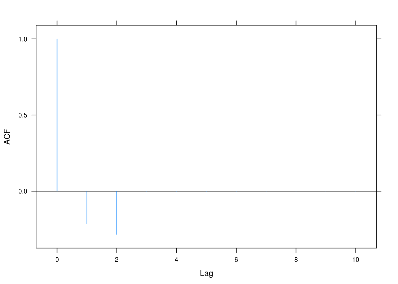
Figure 4.1: Autocorrelation with \(\theta_1 = 0.5\) and \(\theta_2 = 0.4\)
b
tacf(ma = list(-1.2, 0.7))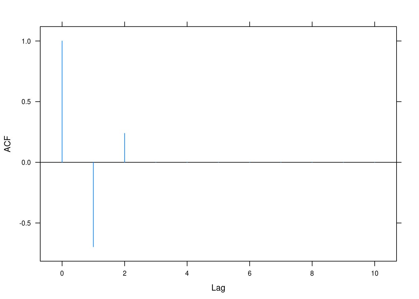
Figure 4.2: Autocorrelation with \(\theta_1 = 1.2\) and \(\theta_2 = -0.7\)
c
tacf(ma = list(1, 0.6))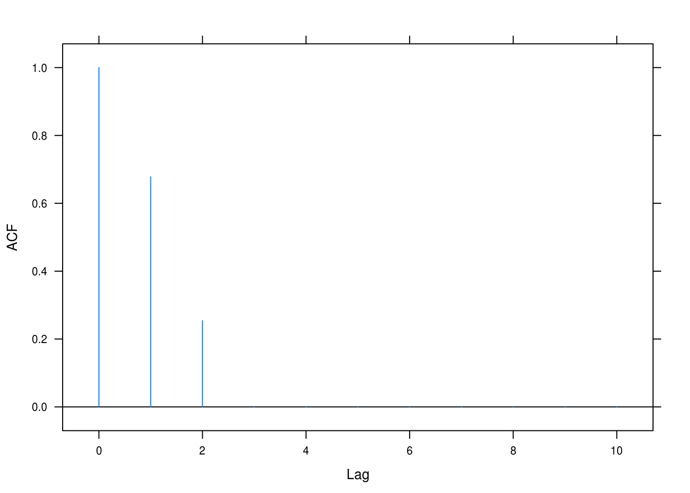
Figure 4.3: Autocorrelation with \(\theta_1 = -1\) and \(\theta_2 = -0.6\)
4.3 Max and min correlations for MA(1)
For \[ \rho_1 = \frac{-\theta}{1+\theta^2} \] we retrieve extreme values at \[ \frac{\partial}{\partial \theta}\rho_1 = \frac{-1(1+\theta^2)-2\theta(-\theta)}{(1+\theta^2)^2} = \frac{\theta^2 - 1}{(1+\theta^2)^2} = 0 \] when \(t = \begin{cases}-1\\1\end{cases}\), which gives us \[ \begin{aligned} \max \rho_1 & = \frac{-1(-1)}{1+(-1)^2} = 0.5\\ \min \rho_1 & = \frac{-1}{1+1^2} = -0.5 \end{aligned} \] which we graph in figure 4.4
theta <- seq(-10, 10, by = 0.01)
p1 <- (-theta) / (1 + theta^2)
plot(theta, p1, type = "l")
points(theta[which.max(p1)], max(p1))
points(theta[which.min(p1)], min(p1))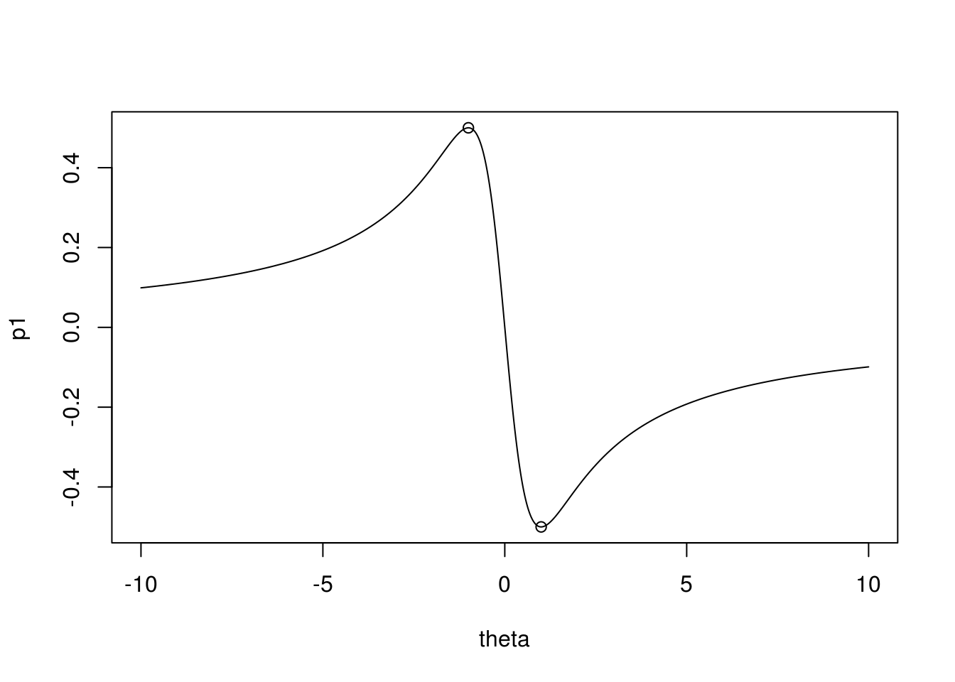
Figure 4.4: Autocorrelation at lag one for MA(1) with max and min annotated.
4.4 Non-uniqueness of MA(1)
\[ \frac{-\frac{1}{\theta}}{1 + \left( \frac{1}{\theta}\right)^2} = \frac{-\frac{1}{\theta}\times\theta^2}{\left( 1 + \frac{1}{\theta^2} \right) \theta^2} = \frac{-\theta}{1+\theta^2} \tag*{$\square$} \]
4.5 Sketch more autocorrelations
theta <- c(0.6, -0.6, 0.95, 0.3)
lag <- c(10, 10, 20, 10)
for (i in seq_along(theta)) {
  print(tacf(ar = theta[i], lag.max = lag[i]))
}
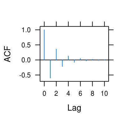
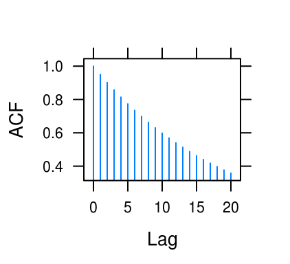
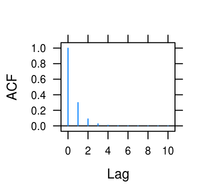
Figure 4.5: ACF for various AR(1) processes.
4.6 Difference function for AR(1)
a
\[ \begin{aligned} \text{Cov}(\triangledown Y_t, \triangledown Y_{t-k}) & = \text{Cov}(Y_t-Y_{t-1}, Y{t-k}-Y_{t-k-1})\\ & = \text{Cov}(Y_t, Y_{t-k}) - \text{Cov}(Y_{t-1},Y_{t-k}) - \text{Cov}(Y_t, Y_{t-k-1}) + \text{Cov}(Y_{t-1}, Y_{t-k-1})\\ & = \frac{\sigma_e^2}{1-\phi^2}(\phi^2 - \phi^{k-1}-\phi^{k+1}+\phi^k) \\ & = \frac{\sigma_e^2}{1-\phi^2}\phi^{k-1}(2\phi-\phi2-1)\\ & = - \frac{\sigma_e^2}{1-\phi^2}(1-\phi)^2\phi^{k-1}\\ & = - \sigma_e^2 \frac{(1-\phi)^2}{(1-\phi)(1+\phi)}\\ & = -\sigma_e^2 \frac{1-\phi}{1+\phi}\phi^{k-1} \end{aligned} \] as required.
b
\[ \begin{aligned} \text{Var}(W_t) & = \text{Var}(Y_t-Y_{t-1})\\ & = \text{Var}(\phi_1Y_{t-1}+e_t-Y_{t-1})\\ & = \text{Var}(Y_{t-1}(\phi-1)+\sigma_e^2)\\ & = (\phi-1)^2\text{Var}(Y_{t-1}) + \text{Var}(e_t)\\ & = \frac{\sigma_e^2}{1-\phi^2}(\phi^2-2\phi+1) + \sigma_e^2\\ & = \frac{\sigma_e^2(\phi^2-2\phi+1+1-\phi^2)}{1-\phi^2}\\ & = \frac{2\sigma_e^2(1-\phi)}{1-\phi^2} \\ & = \frac{2\sigma_e^2}{1+\phi} \tag*{$\square$} \end{aligned} \]
4.7 Characteristics of several models
a
Only correlation at lag 1.
b
Only autocorrelation at lag 1 and 2. Shape of process depends on values of coefficients.
c
Exponentially decaying correlation from lag 0.
d
Different patterns in ACF that depends on whether roots are complex or real.
e
Exponentially decaying correlations from lag 1.
4.8 AR(2)
First, we have variance \[ \text{Var}(Y_t) = \text{Var}(\phi_2 Y_{t-2} + e_t) = \phi_2^2 \text{Var}Y_{t-2} + \sigma_e^2 \] which, assuming stationarity, is equivalent to \[ \text{Var}(Y_{t-2}) = \phi_2^2\text{Var}(Y_{t-2}) + \sigma_e^2 \iff \\ \sigma_e^2 = (1-\phi_2^2) \text{Var}(Y_{t-2}) \iff \\ \text{Var}(Y_{t-2}) = \frac{\sigma_e^2}{1-\phi^2_2} \] which requires that \(-1 < \phi_2 < 1\) since \(\text{Var}(Y_{t-2}) \geq 0\).
4.9 Sketching AR(2) processes
a
\[ \begin{split} \rho_1 & = 0.6\rho_0 + 0.3\rho{-1} = 0.6 + 0.3\rho_1 = 0.8571 \\ \rho_2 & = 0.6\rho_1+0.3\rho_0 = 0.81426\\ \rho_3 & = 0.6\rho_2 + 0.3\rho_1 = 0.7457 \end{split} \]
The roots to the characteristic equation are given by
\[ \frac{\phi_1 \pm \sqrt{\phi_1^2 + 4\phi_2}}{-2\phi_2} = \frac{0.6 \pm \sqrt{0.6 + 4 \times 0.3}}{-2 \times 0.3} = -1 \pm 2.0817 = \{1.0817, -3.0817\}. \]
Since both of these roots exceed 1 in absolute value, they are real. Next, we sketch the theoretical autocorrelation function (4.6).
tacf(ar = c(0.6, 0.3))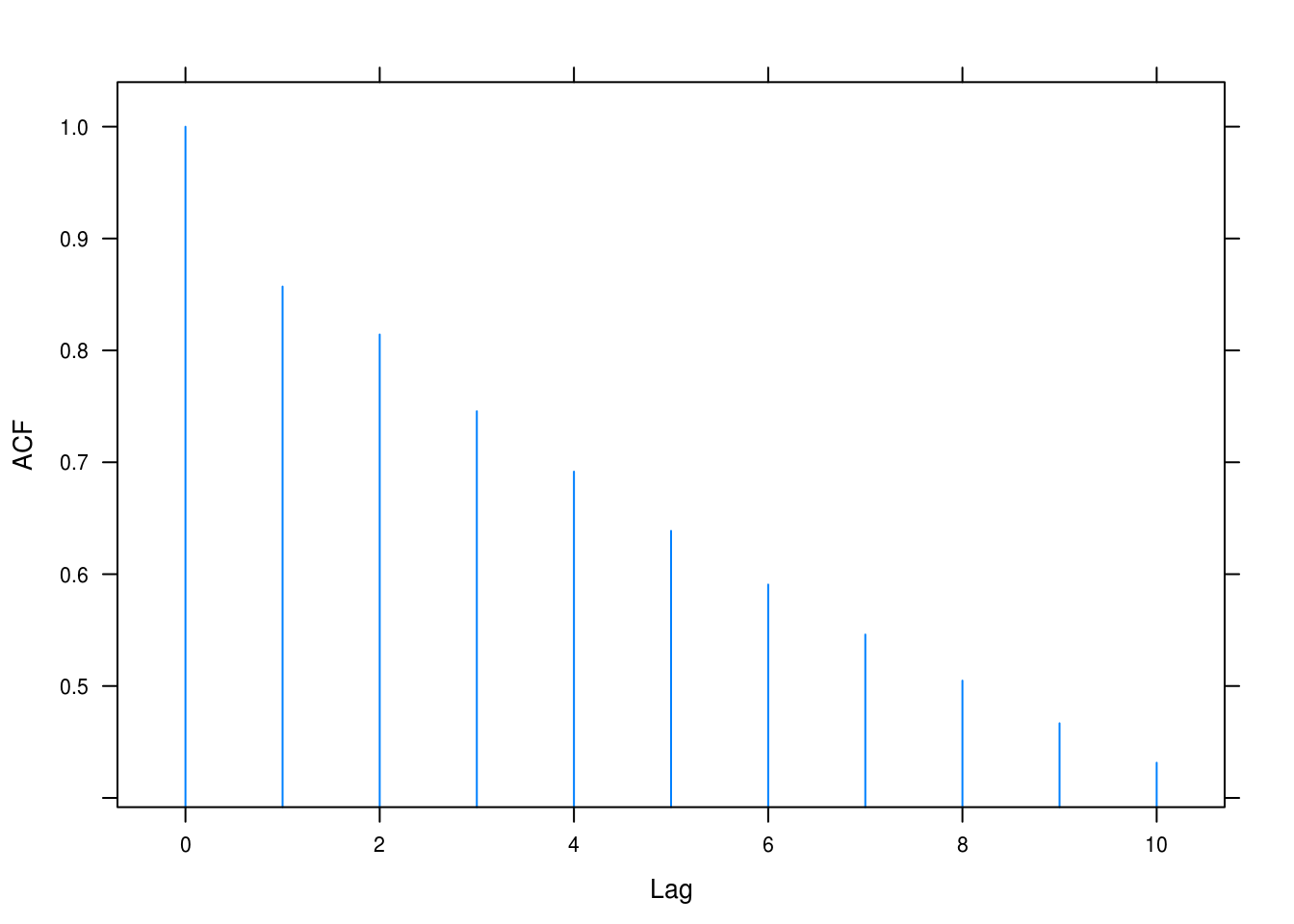
Figure 4.6: ACF for AR(2) with \(\phi_1 = 0.6, \phi_2 = 0.3\).
b
Next we write a function to do the work for us.
ar2solver <- function(phi1, phi2) {
  roots <- polyroot(c(1, -phi1, -phi2))
  cat("Roots:\t\t", roots, "\n")

  if (any(Im(roots) > sqrt(.Machine$double.eps))) {
    damp <- sqrt(-phi2)
    freq <- acos(phi1 / (2 * damp))

    cat("Dampening:\t", damp, "\n")
    cat("Frequency:\t", freq, "\n")
  }

  tacf(ar = c(phi1, phi2))
}ar2solver(-0.4, 0.5)## Roots: -1.1+0i 1.9-0i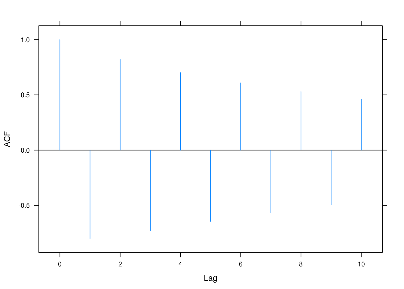
Figure 4.7: ACF for AR(2) with \(\phi_1 = -0.4, \phi_2 = 0.5\).
c
ar2solver(1.2, -0.7)## Roots: 0.86+0.83i 0.86-0.83i
## Dampening: 0.84
## Frequency: 0.77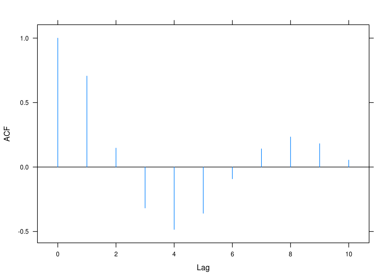
Figure 4.8: ACF for AR(2) with \(\phi_1 = 1.2, \phi_2 = -0.7\).
d
ar2solver(-1, -0.6)## Roots: -0.83+0.99i -0.83-0.99i
## Dampening: 0.77
## Frequency: 2.3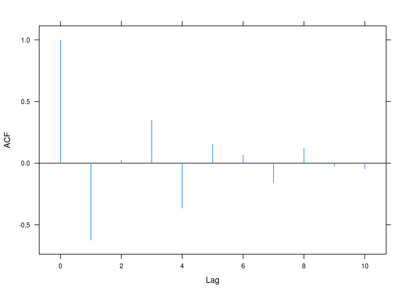
Figure 4.9: ACF for AR(2) with \(\phi_1 = -1, \phi_2 = -0.6\).
e
ar2solver(0.5, -0.9)## Roots: 0.3+1i 0.3-1i
## Dampening: 0.95
## Frequency: 1.3
Figure 4.10: ACF for AR(2) with \(\phi_1 = 0.5, \phi_2 = -0.9\).
f
ar2solver(-0.5, -0.6)## Roots: -0.4+1.2i -0.4-1.2i
## Dampening: 0.77
## Frequency: 1.9
Figure 4.11: ACF for AR(2) with \(\phi_1 = -0.5, \phi_2 = -0.6\).
4.10 Sketch ARMA(1,1) models
a
tacf(ar = 0.7, ma = -0.4)
Figure 4.12: ACF for ARMA(1,1) with \(\phi = 0.7\) and \(\theta = 0.4\).
b
tacf(ar = 0.7, ma = 0.4)
Figure 4.13: ACF for ARMA(1,1) with \(\phi = 0.7\) and \(\theta = -0.4\).
4.11 ARMA(1,2)
a
\[ \begin{aligned} \text{Cov}(Y_t, Y_{t-k}) & = \text{E}[(0.8Y_{t-1}+e_t+0.7e_{t-1}+0.6e_{t-2})Y_{t-k}] - \text{E}(Y_t)\text{E}(Y_{t-k})\\ & = \text{E}(0.8Y_{t-1}Y_{t-k} + Y_{t-k}e_t + 0.7e_{t-1}Y_{t-k}+0.6e_{t-2}Y_{t-k}) - 0\\ & = 0.8\text{E}(Y_{t-1}Y_{t-k}) + \text{E}(Y_{t-k}e_t) + 0.7\text{E}(e_{t-1}Y_{t-k}) + 0.7\text{E}(e_{t-2}Y_{t-k})\\ & = 0.8\text{E}(Y_{t-1}Y_{t-k})\\ & = 0.8\text{Cov}(Y_t,Y_{t-k+1})\\ & = 0.8\gamma_{k-1} & \square \end{aligned} \]
b
\[ \begin{split} \text{Cov}(Y_t,Y_{t-2}) & = \text{E}[0.8Y_{t-1}+e_t+0.7e_{t-1}+0.6e_{t-2})Y_{t-2}]\\ & = \text{E}[(0.8Y_{t-1}+0.6e_{t-2})Y_{t-2}]\\ & = 0.8\text{Cov}(Y_{t-1},Y_{t-2})+0.6\text{E}(e_{t-2}Y_{t-2})\\ & = 0.8\gamma_1 + 0.6\text{E}(e_t Y_t)\\ & = 0.8\gamma_1 + 0.6\text{E}[e_t(0.8Y_{t-1}+e_t+0.7e_{t-1}+0.6e_{t-2})]\\ & = 0.8\gamma_1 + 0.6\sigma_e^2 \iff \\ \rho_2 & = 0.8\rho_1+0.6\sigma_e^2/\gamma_0 & \square \end{split} \]
4.12 Two MA(2) processes
a
For \(\theta_1 = \theta_2 = 1/6\) we have \[ \rho_k = \frac{-\frac{1}{6}+\frac{1}{6}\times\frac{1}{6}}{1 + \left(\frac{1}{6}\right)^2 + \left(\frac{1}{6}\right)^2} = \frac{\frac{1}{6}\left(\frac{1}{6}-1\right)}{1 + \frac{2}{36}} = - \frac{5}{38}. \]
For \(\theta_1 = -1\) and \(\theta_2 = 6\), \[ \rho_k = \frac{1-6}{1+1^2+36} = - \frac{5}{38} \tag*{$\square$}. \]
b
For \(\theta_1 = \theta_2 = 1/6\) we have roots given by \[ \frac{\frac{1}{6} \pm \sqrt{\frac{1}{36}+ 4 \times \frac{1}{6}}}{-2\times \frac{1}{6}} = - \frac{1}{2} \pm \frac{\sqrt{\frac{25}{36}}}{-\frac{1}{3}} = - \frac{1}{2} \pm \frac{\frac{5}{6}}{\frac{1}{3}} = \{-3, -2\} \]
and for \(\theta_1 = -1\) and \(\theta_2 = 6\), \[ \frac{-1 \pm \sqrt{1 + 4 \times 6}}{-2\times6} = \frac{-1\pm 5}{-12} = \frac{1}{12} \pm \frac{5}{12} = \left\{-\frac{1}{3}, \frac{1}{2}\right\} \]
4.13 Autocorrelation in MA(1)
\[ \begin{aligned} & \text{Var}(Y_{n+1}+Y_n+Y_{n-1}+ \dots + Y_1) = \left((n+1)+2n\rho_1\right)\gamma_0 = \left(1+n(1+2\rho_1)\right)\gamma_0\\ & \text{Var}(Y_{n+1}-Y_n+Y_{n-1}- \dots + Y_1) = \left((n+1)-2n\rho_1 \right)\gamma_0 = \left(1 + n(1-2\rho_1)\right)\gamma_0 \end{aligned} \]
[ \begin{cases} \left(1+n(1+2\rho-1)\right) \geq 0 \\ \left(1+n(1-2\rho-1)\right) \geq 0 \\ \end{cases} \begin{cases} 1+n+2\rho_1n \geq 0 \\ 1+n-2\rho_1n \geq 0 \\ \end{cases} \begin{cases} \rho_1 \geq \frac{-(n+1)}{2n}\\ \rho_1 \leq \frac{n+1}{2n} \end{cases} \begin{cases} \rho_1 \geq -\frac{1}{2}(1+\frac{1}{n})\\ \rho_1 \leq \frac{1}{2}(1+\frac{1}{n}) \end{cases}] where \(\rho_1 \geq |1/2|\) for all \(n\).
4.14 Zero-mean stationary process
We set \(Y_t=e_t−θe_t−1\) and then we have
\[ \begin{split} e_t & = \sum_{j=0}^\infty \theta^j Y_{t-j}\quad \text{and expanding into} \\ & = \sum_{j=1}^\infty \theta^j Y_{t-j} + \theta^0 Y_{t-0} \\ & \iff \\ Y_t & = e_t - \sum_{j=1}^\infty \theta^j Y_{t-j} \end{split} \] which is equivalent to \[ Y_t = \mu_0 + (1 + \theta B + \theta^2 B^2 + \dots + \theta^n B^n)e_t \] which is the definition of a MA(1) process where \(B\) is the backshift operator such that \(Y_t B^k =Y_{t-k}\).
4.15 Stationarity prerequisite of AR(1)
\[ \begin{split} \text{Var}(Y_t) & = \text{Var}(\phi Y_{t-1}+e_t) = \phi^2\text{Var}(Y_{t-1})+\sigma_e^2\\ & = \phi^2 \text{Var}(\phi Y_{t-2}+e_t)+\sigma_e^2\\ & = \phi^4 \text{Var}(Y_{t-2})+2\sigma_e^2\\ & = \phi^{2n}\text{Var}(Y_{t-n})+n\sigma_e^2 \end{split} \] And \(\lim_{n \rightarrow \infty} \text{Var}(Y_t) = \infty\) if \(|\phi\)=1$, which is impossible.
4.16 Nonstationary AR(1) process
a
\[ \begin{split} Y_t & = \phi Y_{t-1}+e_t \implies \\ - \sum_{j=1}^\infty \left(\frac{1}{3}\right)^j e_{t+j} & = 3 \left(-\sum_{j=1}^\infty \left(\frac{1}{3}\right)^j e_{t-1+j}\right) + e_t\\ - \sum_{j=1}^\infty \left(\frac{1}{3}\right)^{j+1} e_{t+j} & = -\sum_{j=1}^\infty \left(\frac{1}{3}\right)^j e_{t-1+j} + \frac{1}{3} e_t\\ - \sum_{j=1}^\infty \left(\frac{1}{3}\right)^{j+1} e_{t+j} & = -\sum_{j=2}^\infty \left(\frac{1}{3}\right)^j e_{t-1+j}\\ - \sum_{j=1}^\infty \left(\frac{1}{3}\right)^{j+1} e_{t+j} & = -\sum_{j+1=2}^\infty \left(\frac{1}{3}\right)^{j+1} e_{t+j} & \square \end{split} \]
b
\[ \text{E}(Y_t) = \text{E}(\sum_{j=1}^\infty \left(\frac{1}{3}\right)^j e_{t+j}) = 0 \] since all terms are uncorrelated white noise.
\[ \begin{gathered} \text{Cov}(Y_t,Y_{t-1}) = \text{Cov}\left( -\sum_{j=1}^\infty \left(\frac{1}{3}\right)^j e_{t+j}, \sum_{j=1}^\infty \left(\frac{1}{3}\right)^j e_{t+j-1} \right) = \\ \text{Cov}\left(-\frac{1}{3}e_{t+1} - \left(\frac{1}{3}\right)^2e_{t+2} - \dots - \left(\frac{1}{3}\right)^n e_{t+n}, -\frac{1}{3}e_{t} - \left(\frac{1}{3}\right)^2e_{t+1} - \dots - \left(\frac{1}{3}\right)^n e_{t+n-1} \right) = \\ \text{Cov}\left(-\frac{1}{3}e_{t+1},-\frac{1}{3^2}e_{t+1}\right) + \text{Cov}\left(-\frac{1}{3}e_{t+2},-\frac{1}{3^3}e_{t+2}\right) + \dots + \text{Cov}\left(-\frac{1}{3}e_{t+n},-\frac{1}{3^{n+1}}e_{t+n}\right) = \\ \frac{1}{26}\sigma_e^2\left(1 + \frac{1}{3} + \frac{1}{3^2} + \dots + \frac{1}{3^n} \right) \end{gathered} \] which is free of \(t\).
c
It is unsatisfactory because Y_t depends on future observations.
4.17 Solution to AR(1)
a
\[ \frac{1}{2}\left(10\left(\frac{1}{2}\right)^{t-1} + e_{t-1} + \frac{1}{2}e_{t-2} + \left(\frac{1}{2}\right)^2e_{t-3} + \dots + \left(\frac{1}{2}\right)^{n-1}e_{t-n}\right) + e_{t-1} = \\ 10 \left(\frac{1}{2}\right)^t + \frac{1}{2}e_{t-1} + \left(\frac{1}{2}\right)^2e_{t-2} + \left(\frac{1}{2}\right)^3 e_{t-3} + \dots + \left( \frac{1}{2}\right)^n e_{t-n} + e_{t-1} = \\ 10\left(\frac{1}{2}\right)^{t-1} + e_{t-1} + \frac{1}{2}e_{t-2} + \left(\frac{1}{2}\right)^2e_{t-3} + \dots + \left(\frac{1}{2}\right)^{n-1}e_{t-n} \qquad \square \]
b
\(\text{E}(Y_t) = 10 \left( \frac{1}{2}\right)^t\) varies with \(t\) and thus is not stationary.
4.18 Stationary AR(1)
a
\[ \text{E}(W_t) = \text{E}(Y_t + c\phi^t) = \text{E}(Y_t) + \text{E}(c\phi^t) = 0 + c\phi^t = c\phi^t \tag*{$\square$} \]
b
\[ \phi(Y_{t-1}+c\phi^{t-1})+e_t = \phi Y_{t-1} + c\phi^t + e_t = \phi \left( \frac{Y_t - e_t}{\phi}\right) + c \phi^t + e_t = Y_t + c\phi^t \tag*{$\square$} \]
c
No, (W_t) is not free of \(t\).
4.19 Find a simpler model (1)
This is similar to an AR(1) with \(\rho_k = -(-0.5)^k\).
ARMAacf(ar = -0.5, lag.max = 7)## 0 1 2 3 4 5 6 7
## 1.0000 -0.5000 0.2500 -0.1250 0.0625 -0.0312 0.0156 -0.0078ARMAacf(ma = -c(0.5, -0.25, 0.125, -0.0625, 0.03125, -0.0015625))## 0 1 2 3 4 5 6 7
## 1.0000 -0.4997 0.2492 -0.1232 0.0589 -0.0240 0.0012 0.00004.20 Find a simpler model (2)
This is like an ARMA(1,1) with \(\phi = -0.5\) and \(\theta = 0.5\).
[ \begin{cases} \psi_1 = \phi - \theta = 1\\ \psi_2 = (\phi - \theta)\phi = -0.5 \end{cases} \begin{cases} \theta = 0.5\\ \phi = -0.5 \end{cases}]
ARMAacf(ma = -c(1, -0.5, 0.25, -0.125, 0.0625, -0.03125, 0.015625))## 0 1 2 3 4 5 6 7 8
## 1.0000 -0.7142 0.3570 -0.1783 0.0887 -0.0435 0.0201 -0.0067 0.0000ARMAacf(ar = -0.5, ma = -0.5, lag.max = 8)## 0 1 2 3 4 5 6 7 8
## 1.0000 -0.7143 0.3571 -0.1786 0.0893 -0.0446 0.0223 -0.0112 0.00564.21 ARMA in disguise
a
\[ \begin{gathered} \text{Cov}(Y_t, Y_{t-k}) = \text{Cov}(e_{t-1}-e_{t-2}+0.5e_{t-3}, e_{t-1-k}-e_{t-2-k}+0.5e_{t-3-k}) = \\ \gamma_k = \begin{cases} \sigma_e^2 + \sigma_e^2 + 0.25\sigma_e^2 = 2.25\sigma_e^2 & k = 0\\ -\sigma_e^2-0.5\sigma_e^2=-1.5\sigma_e^2 & k = 1\\ 0.5\sigma_e^2 & k = 2 \end{cases} \end{gathered} \]
b
This is an ARMA(p,q) in the sense that \(p = 0\) and \(q = 2\), that is, it is in fact an MA(2) process \(Y_t = e_t - e_{t-1}+0.5e_{t-2}\) with \(\theta_1 = 1, \theta2 = -0.5\).
4.22 Equivalence of statements
\[ 1 - \phi_1x - \phi_2x^2 - \dots - \phi_p x^p \implies x^k \left( \left(\frac{1}{k}\right)^p - \phi_1 \left(\frac{1}{k}\right)^{p-1} \dots - \phi_p \right) \]
Thus if \(x_1 = G\) is a root to the above, \(\frac{1}{x_1} = \frac{1}{G}\) must be a root to \[ x^p - \phi_1 x^{p-1} -\phi_2 x^{p-2} - \dots -\phi_p \]
4.23 Covariance of AR(1)
a
\[ \begin{gathered} \text{Cov}(Y_t - \phi Y_{t+1}, Y_{t-k} - \phi Y_{t-k+1}) = \\ \text{Cov}(Y_t, Y_{t-k}) - \phi \text{Cov}(Y_t, Y_{t+1-k}) - \phi\text{Cov}(Y_{t+1},Y_{t-k}) + \phi^2\text{Cov}(Y_{t+1, Y_{t+1-k}}) = \\ \frac{\sigma_e^2}{1-\phi^2}\left(\phi^k - \phi \phi^{k-1} - \phi \phi^{k+1} + \phi^2 \phi\right) =\\ \frac{\sigma_e^2}{1-\phi^2}\left( \phi^k - \phi^k - \phi^{k+2} + \phi^{k+2} \right) = 0 \end{gathered} \]
b
First,
\[ Y_{t+k} = \phi Y_{t+k-1} + e_t + k \implies \]
\[ \begin{split} \text{Cov}(b_t, Y_{t+k}) & = \text{Cov}(Y_t - \phi Y_{t+1, Y_{t+n}})\\ & = \text{Cov}(Y_t,Y_{t+k}) - \phi \text{Cov}(Y_{t+1}, Y_{t+k)})\\ & = \frac{\sigma_e^2}{1-\phi^2}\phi^k - \phi \frac{\sigma_e^2}{1-\phi^2}\phi^{k-1}\\ & = 0 & \square \end{split} \]
4.24 Recursion
a
\[ \begin{split} E(Y_0) & = E[c_1e_0] = c_1E[e_0] = 0\\ E(Y_1) & = E(c_2Y_0 + e_1) = c_2 E(Y_0) = 0\\ E(Y_2) & = E(\phi_1 Y_1 + \phi_2 Y_0 + e_t) = 0\\ & \vdots \\ E(Y_t) & = E(\phi_1 Y_{t-1} + \phi_2 Y_{t-2}) = 0 \end{split} \]
b
We have \[ \begin{cases} \text{Var}(Y_0) = c_1^2\text{Var}(e_0) = c_1^2\sigma_e^2\\ \text{Var}(Y_1) = c_2^2\text{Var}(Y_0) + \text{Var}(e_0) = c_2^2c_1^2\sigma_e^2=\sigma_e^2(1+c_1^2c_2^2) \end{cases} \implies \]
\[ \begin{cases} c_1^2\sigma_e^2 = \sigma_e^2(1+c_1^2c_2^2) & \iff c_1^2(1-c_2^2) = 1\\ c_1^2 = \frac{1}{1-c_2^2} & \iff c_1 = \sqrt{\frac{1}{1-c_1^2}} = \frac{1}{\sqrt{1-c_1^2}} \end{cases} \] with covariance \[ \begin{gathered} \text{Cov}(Y_0, Y_1) = \text{Cov}(c_1e_0,c_2 c_1 e_0 + e_1) = \text{Cov}(c_1e_0,c_2 c_1 e_0) + \text{Cov}(c_1e_0, e_1) =\\ c_1^2c_2\sigma_e^2 + c_1\text{Cov}(e_0, e_1) = c_1^2c_2\sigma_e^2 + 0 \end{gathered} \] and autocorrelation \[ \rho_1 = \frac{c_1^2c_2\sigma_e^2}{\sqrt{(c_1^2)^2}} = c_2 \] so we must choose \[ \begin{cases} c_2 = \frac{\phi_1}{1-\phi_2} \\ c_1 = \frac{1}{\sqrt{1-c_2^2}} \end{cases}. \]
c
The process can be transformed by scaling and standardizing it and then shifting with any given mean. \[ \frac{Y_t \sqrt{y_0}}{c_1} + \mu \]
4.25 Final exercise
a
\[ \begin{split} Y_t & = \phi Y_{t-1} + e_t\\ & = \phi(\phi Y_{t-2}+e_{t-1}) + e_t = \phi^2 Y_{t-2} + \phi e_{t-1} + e_t\\ & \vdots \\ & = \phi^t Y_{t-t} + \phi e_{t-1} + \phi^2 e_{t-2} + \dots + \phi^{t-1}e_1+e_t & \square \end{split} \]
b
\[ E(Y_t) = E(\phi^t Y_0 +\phi e_{t-1} + \phi^2 e_{t-2} + \dots + \phi^{t-1}e_1+e_t) =\phi^t\mu_0 \]
c
\[ \begin{split} \text{Var}(Y_t) & = \text{Var}(\phi^t Y_0 + \phi e_{t-1}+\phi^2e_{t-2} + \dots + \phi^{t-1}e_1)\\ & = \phi^{2t}\sigma_0^2+\sigma_e^2 \sum_{k=0}^{t-1}(\phi^2)^k\\ & = \sigma_e^2 \frac{1-\phi^{2n}}{1-\phi^2} + \phi^{2t}\sigma_0^2 \quad\text{if $\phi \neq 1$ else}\\ & = \text{Var}(Y_0) + \sigma_e^2 t = \sigma_0^2 + \sigma_e^2 t \end{split} \]
d
If \(\mu_0 = 0\) then \(E(Y_t) = 0\) but for \(\text{Var}(Y_t)\) to be free of t, \(\phi\) cannot be 1.
e
\[ \text{Var}(Y_t) = \phi^2 \text{Var}(Y_{t-1}) + \sigma_e^2 \implies \phi^2 \text{Var}(Y_t) + \sigma_e^2 \] and \[ \text{Var}(Y_{t-1}) = \text{Var}(Y_t)(1-\phi^2) = \sigma_e^2 \implies \text{Var}(Y_t) = \frac{\sigma_e^2}{1-\phi} \]
and then we must have \(|\phi| < 1\).