Plot Coefficients

Plot the fitted model's regression coefficients along the regularization path. When the path contains a single solution (only one alpha value), a dot chart is displayed showing the coefficient values. When the path contains multiple solutions, a line plot is displayed showing how coefficients evolve along the regularization path.

Usage

# S3 method for class 'SLOPE'
plot(
  x,
  intercept = FALSE,
  x_variable = c("alpha", "deviance_ratio", "step"),
  magnitudes = FALSE,
  add_labels = FALSE,
  mark_zero = TRUE,
  ...
)

Arguments

x

an object of class "SLOPE"

intercept

whether to plot the intercept

x_variable

what to plot on the x axis. "alpha" plots the scaling parameter for the sequence, "deviance_ratio" plots the fraction of deviance explained, and "step" plots step number.

magnitudes

whether to plot the magnitudes of the coefficients

add_labels

whether to add labels (numbers) on the right side of the plot for each coefficient (only used when the path contains multiple solutions)

mark_zero

whether to add a vertical line at zero in the dot chart (only used when the path contains a single solution)

...

for multiple solutions: arguments passed to graphics::matplot(). For a single solution: arguments passed to graphics::dotchart().

Value

Invisibly returns NULL. The function is called for its side effect of producing a plot.

See also

SLOPE(), plotDiagnostics()

Other SLOPE-methods: coef.SLOPE(), deviance.SLOPE(), predict.SLOPE(), print.SLOPE(), score(), summary.SLOPE()

Examples

# Multiple solutions along regularization path
fit <- SLOPE(heart$x, heart$y)
plot(fit)


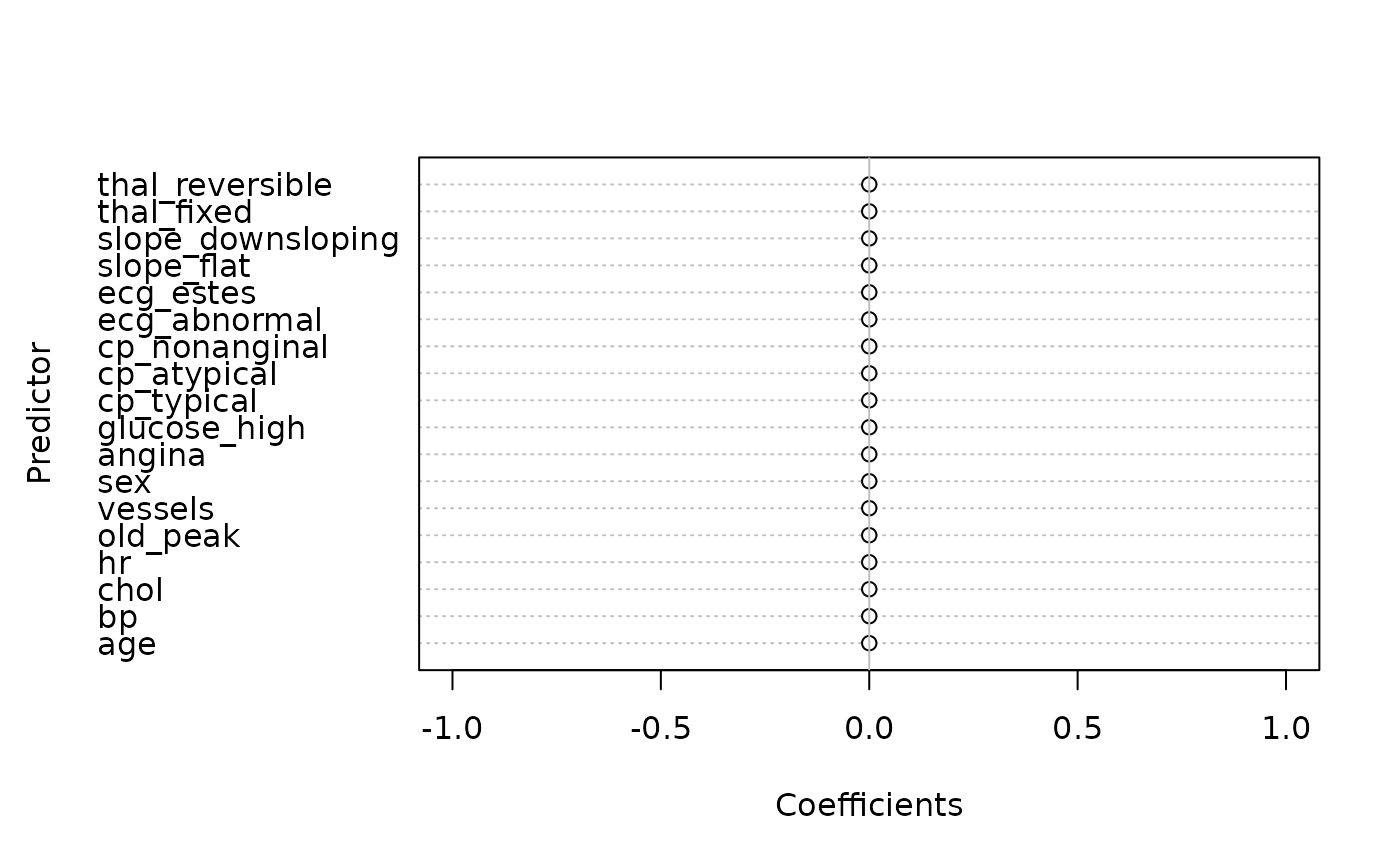
# Single solution with dot chart
fit_single <- SLOPE(heart$x, heart$y, alpha = 0.1)
plot(fit_single)


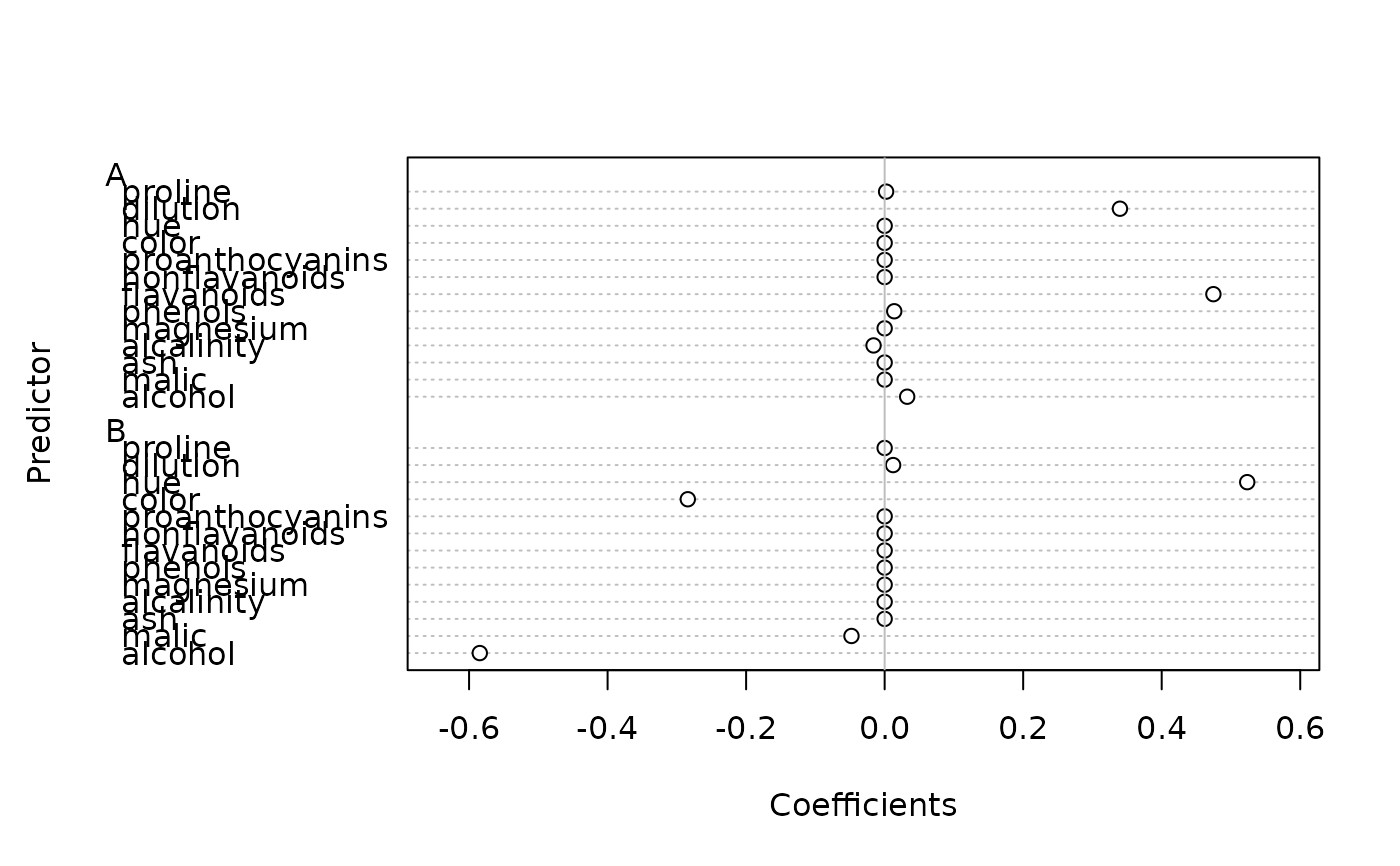
# Single solution for multinomial regression
fit_multi <- SLOPE(wine$x, wine$y, family = "multinomial", alpha = 0.05)
plot(fit_multi)