Background
sgdnet uses the incremental gradient method SAGA (Defazio, Bach, and Lacoste-Julien 2014), which is a modification of the Stochastic Average Gradient (SAG) algorithm introduced in Schmidt, Roux, and Bach (2017). SAGA handles both strongly and non-strongly convex objectives – even in the composite case – making it applicable to a wide range of problems such as generalized linear models with elastic net regularization (Zou and Hastie 2005), which is the problem that sgdnet is designed to handle.
SAGA has a simple convergence proof and uses a step size that in fact adjusts automatically to the magnitude of strong convexity in the objective. This makes it practical for the end user, who avoids having to tune step size by hand.
The purpose of this vignette is to present the algorithm as it is implemented in sgdnet and to serve as guidance for anyone who is interested contributing to the development of the package.
Model setup
Before the algorithm is set loose on data, its parameters have to be set up properly and its data (possibly) preprocessed. For illustrative purposes, we will proceed by example and use Gaussian univariate regression on the trees dataset. We will attempt to predict the volume of a tree based on girth and height.
Standardization
By default, the feature matrix in sgdnet is centered and scaled to unit variance1.
sgdnet_sd <- function(x) sqrt(sum((x - mean(x))^2)/length(x))
n <- nrow(x)
x_bar <- colMeans(x)
x_sd <- apply(x, 2, sgdnet_sd)
x <- scale(x, center = x_bar, scale = x_sd)
In the univariate Gaussian case, we also standardize the response.
Regularization path
sgdnet supports \(\ell_1\)- and \(\ell_2\)-regularized regression as well as the elastic net, which is a linear combination of the two that is controlled by \(\alpha\), such that
\[\alpha = \frac{\lambda_2}{\lambda_1 + \lambda_2}\]
where \(\lambda_1\) and \(\lambda_2\) denotes the amount of \(\ell_1\) and \(\ell_2\) regularization respectively.
For our example, let’s say that we are fitting the elastic net with \(\alpha = 0.5\).
Typically, we fit a model along a path of \(\lambda\), beginning with \(\lambda_{max}\): the \(\lambda\) at which the solution is completely sparse (save for the intercept, which is not regularized). It can be shown that
\[\lambda_{\text{max}} = \max_{i}\frac{\langle\mathbf{x}_i, \mathbf{y}\rangle}{n\alpha}\] Of course, when \(\alpha = 0\) as in ridge regression, this value becomes undefined and so we constrain it so that \(\alpha \geq 0.001\) in the computation of \(\lambda_{\text{max}}\).
For our example, we get the following.
We then construct the \(\lambda\) path to be a \(\log_e\)-spaced sequence starting at \(\lambda_{\text{max}}\) and finishing at \(\lambda_{\text{max}} \times \lambda_{\text{min ratio}}\). Thus we have
lambda.min.ratio <- 0.01
nlambda <- 100
lambda <- exp(seq(log(lambda_max),
                  log(lambda_max*lambda.min.ratio),
                  length.out = nlambda))
head(lambda)
#> [1] 1.934239 1.846325 1.762406 1.682302 1.605839 1.532851
lambda.min.ratio and nlambda are both setable through the API, but are given here at their defaults (per this example). Note that we return the lambda path on the original scale of the respone, \(\mathbf{y}\), which means that the user sees
lambda_out <- lambda*y_sd
head(lambda_out)
#> [1] 31.27770 29.85608 28.49907 27.20375 25.96729 24.78704
Naturally, whatever value the user provides in the argument lambda to sgdnet() will be scaled accordingly.
Step size
The step size, \(\gamma\), in SAGA is constant throughout the algorithm. For non-strongly convex objectives it is set to \(1/(3L)\), where \(L\) is the maximum Lipschitz constant of the term of the log-likelihood corresponding to a single observation. This is bound to be largest sample-wise squared norm of the feature matrix. For strongly convex objectives, the step size is set to
\[ \frac{1}{3(\mu n + L)},\]
where \(\mu\) is the level of strong convexity and \(n\) the number of samples. For our purposes, \(\mu\), is simply the regularization strength of the \(\ell_2\)-penalty: \(\alpha\lambda\). This has the effect of letting the step size adapt to the type of regularization penalty used.
In our example, where we have the elastic net penalty, we will have the following step sizes (one for each \(\lambda\)). For the sake of illustration, we will also include the case of ridge and lasso penalties to see the differences in step size.
reg <- sapply(c(0, 0.5, 1), function(alpha_i) {
  lambda_2 <- (1 - alpha_i)*lambda/n # l2 penalty
  L <- max(rowSums(x^2)) + lambda_2
  n <- nrow(x)
  mu <- 2*lambda_2
  step_size <- 1 / (2*(L + pmin(mu*n, L)))
})
reg <- as.data.frame(reg)
colnames(reg) <- c("ridge", "elastic_net", "lasso")

library(lattice)
xyplot(ridge + elastic_net + lasso ~ seq_len(nlambda),
       data = reg, type = "l",
       xlab = NULL,
       ylab = expression(gamma),
       auto.key = list(lines = TRUE, points = FALSE, space = "right"))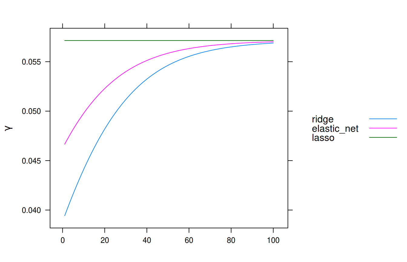
Step sizes along the regularization path.
Algorithm
We will now look at the implementation (in pseudocode) of the actual SAGA algorithm as it is realized in sgdnet.
y           response vector of size n
X           feature matrix of size n*p, each sample X[j] is stored columnwise
beta        vector of coefficients of size p
g_avg       gradient average
l1          amount of L1-regularization
l2          amount of L2-regularization
max_iter    maximum number of outer iterations
gamma       the step size

for i in 1:max_iter
  for k in 1:n_samples
    X[j] <- draw a sample randomly from X

    # Compute the conditional mean given X[j]
    E[X] <- DotProduct(beta_scale*beta, X[j])

    g_old    <- g[j]
    g_new    <- Gradient(E[X], y)
    g_change <- g_old - g_new

    # Perform l2-regularization by scaling beta
    beta_scale <- beta_scale*(1 - gamma*l2)
    beta <- beta[nz] - g_change*gamma/beta_scale

    # The gradient average step
    X[j] <- Update(k + 1,
                   nz,
                   X[j],
                   g_avg,
                   l1*gamma/beta_scale,
                   gamma/beta_scale)

    # Update gradient average
    g_avg <- g_avg + g_change/n_samples

  # At the end of each epoch, reset the scale and unlag all the coefficients
  beta <- beta*beta_scale
  beta_scale <- 1

  # Check convergence
  if (MaxChange(beta)/Max(beta) < thresh)
    stop # algorithm has converged
From this description we have left out the case where the scale of the coefficients becomes small enough to risk underflow and loss of numerical precision. In this case we simply rescale the coefficients back to their real scale (using beta_scale) and update all the coeffiecients that are lagging behind (if we have sparse features; see below for more information on this).
The algorithm for dense input is relatively straightforward. We
- pick a sample uniformly at random,
- compute the gradient at the current sample,
- make the SAGA update to the coefficients using the gradient average, and
- update the gradient average.
Rinse and repeat until our convergence criterion is met.
Sparse features
The implementation for sparse input, however, is slightly more intricate. The reason is that we can save considerable time by postponing the updates of coefficients when their corresponding features are sparse in the current sample. These “missed” or “lagged” updates can then be updated just-in-time when a sample is drawn that have non-sparse features corresponding to these coefficients or at the end of an epoch, at which point we make sure to update all of the coefficients to be able to check for convergence.
These lagged updates are accomplished in a LaggedUpdate() function, which relies on the following two objects:
lag_scaling- a vector storing the the cumulative geometric sums of the updates to the scale of the coefficients.
lag- a vector of indices indicating which iteration the feature was last updated at.
The definition of LaggedUpdate() is, roughly,
LaggedUpdate(k,                   # iteration
             nz,                  # nonzero indices in current sample
             beta,                # coefficients
             g_avg,               # gradient average
             prox_step_size
             grad_step_size
             lag,
             lag_scaling) {

  for i in 1:length(nz)
    ind <- nz[i] # index of nonzero feature
    missed_updates <- k - lag[ind]

    # L2-regularization
    beta[ind] <- beta[ind] + grad_step_size*lag_scaling[missed_updates]*g_avg[ind]

    # L1-regularization through SoftMax function.
    beta[ind] <- SoftThreshold(beta[ind],
                               prox_step_size*lag_scaling[missed_updates])

    lag[ind] <- k
}
where
Unstandardization
Coefficients from sgdnet are, irrespective of any internal standardizaton, always returned on the scale of the original data. Given our assumed model, we have.
\[\text{E}[\mathbf{Y}] = \beta_0 + \sum_{i=1}^p \beta_i\mathbf{x}_i\]
Using a standardized response and standardized features, we get the following estimation
\[ \frac{\hat{y} - \bar{y}}{s_y} = \hat{\beta}_0 + \sum_{i=1}^p \hat{\beta}_i \left( \frac{\mathbf{x}_i - \bar{x}_i}{s_{x_i}} \right), \]
from which we retrieve the unstandardized intercept
\[ \hat{\beta}_{0_\text{unstandardized}} = \hat{\beta}_0 s_y + \bar{y} - \sum_{i=1}^p \hat{\beta}_i \frac{s_y}{s_{x_i}}\bar{x}_i \]
\[ \hat{\beta}_{i_\text{unstandardized}} = \hat{\beta}_i \frac{s_y}{s_{x_i}} \]
References
Defazio, Aaron, Francis Bach, and Simon Lacoste-Julien. 2014. “SAGA: A Fast Incremental Gradient Method with Support for Non-Strongly Convex Composite Objectives.” In Advances in Neural Information Processing Systems 27, 2:1646–54. Montreal, Canada: Curran Associates, Inc.
Schmidt, Mark, Nicolas Le Roux, and Francis Bach. 2017. “Minimizing Finite Sums with the Stochastic Average Gradient.” Mathematical Programming 162 (1-2): 83–112. https://doi.org/10/f9xwpn.
Zou, Hui, and Trevor Hastie. 2005. “Regularization and Variable Selection via the Elastic Net.” Journal of the Royal Statistical Society. Series B (Statistical Methodology) 67 (2): 301–20.
Here we use the sample standard deviation, dividing by \(n\) rather than \(n-1\), since we are only interested in the sample at hand and not the entire population.↩