An Introduction to sgdnet

Background and motivation

The goal of sgdnet is to be a one-stop solution for fitting elastic net-penalized generalized linear models in the \(n \gg p\) regime. This is of course not novel in and by itself. Several packages, such as the popular glmnet package (Friedman, Hastie, and Tibshirani 2010), already exists to serve this pupose. With sgdnet, however, we set out to improve upon the existing solutions in a number of ways:

fit generalized linear models using the efficient SAGA algorithm (Defazio, Bach, and Lacoste-Julien 2014), which promises to outperform the coordinate descent method that is commonly used to fit the elastic net,
craft a well-documented and accessible codebase to promote collaboration and review, and
implement a general framework in which additional model families, proximal operators, and other algorithms could be incorporated.

sgdnet has on purpose been created to mimic the interface of glmnet. Transitioning between the two is a breeze.

In this vignette, we will look at the basics of fitting a model and reviewing the results of it.

Fitting a model

We will look at Edgar Anderson’s well-known iris data set, giving the measurements of petal and sepal length and width of three species of iris flowers. Our objective will be to predict the species of the flower. First, we’ll split the set into a training set.

train_ind <- sample(nrow(iris), floor(0.8*nrow(iris))) # an 80/20 split
iris_train <- iris[train_ind, ]
iris_test <- iris[-train_ind, ]

We fit the model by specifying our feature matrix to argument x and our response to y, using family = "multinomial" to specify the type of model we would like to fit.

The elastic net mixing parameter in sgdnet is specified via the alpha argument, where a value of 1 imposes the lasso (\(\ell_1\)) penalty, and 0 the ridge (\(\ell_2\)) penalty. For this example, we’ll stick with the default (alpha = 1, the lasso).

library(sgdnet)
fit <- sgdnet(iris_train[, 1:4],       # predictor matrix
              iris_train$Species,      # response
              family = "multinomial",  # model family
              alpha = 1)               # elastic net mixing parameter (default)

The regularization strength is specified via the lambda argument. A high value will impose a larger penalty. We did not specify it here, nor do we need to as sgdnet takes care of fitting our model along a regularization path of different \(\lambda\) values, starting at the value at which the solution is expected to be completely sparse, that is, the point at which all coefficients (save for the intercept if it is included) are zero.

Plotting the fit

The result can be printed, which will show a summary of the deviance ratio of the model along the regularization path. Usually, however, it is more effective to study the fit by visualizing it.

plot(fit)

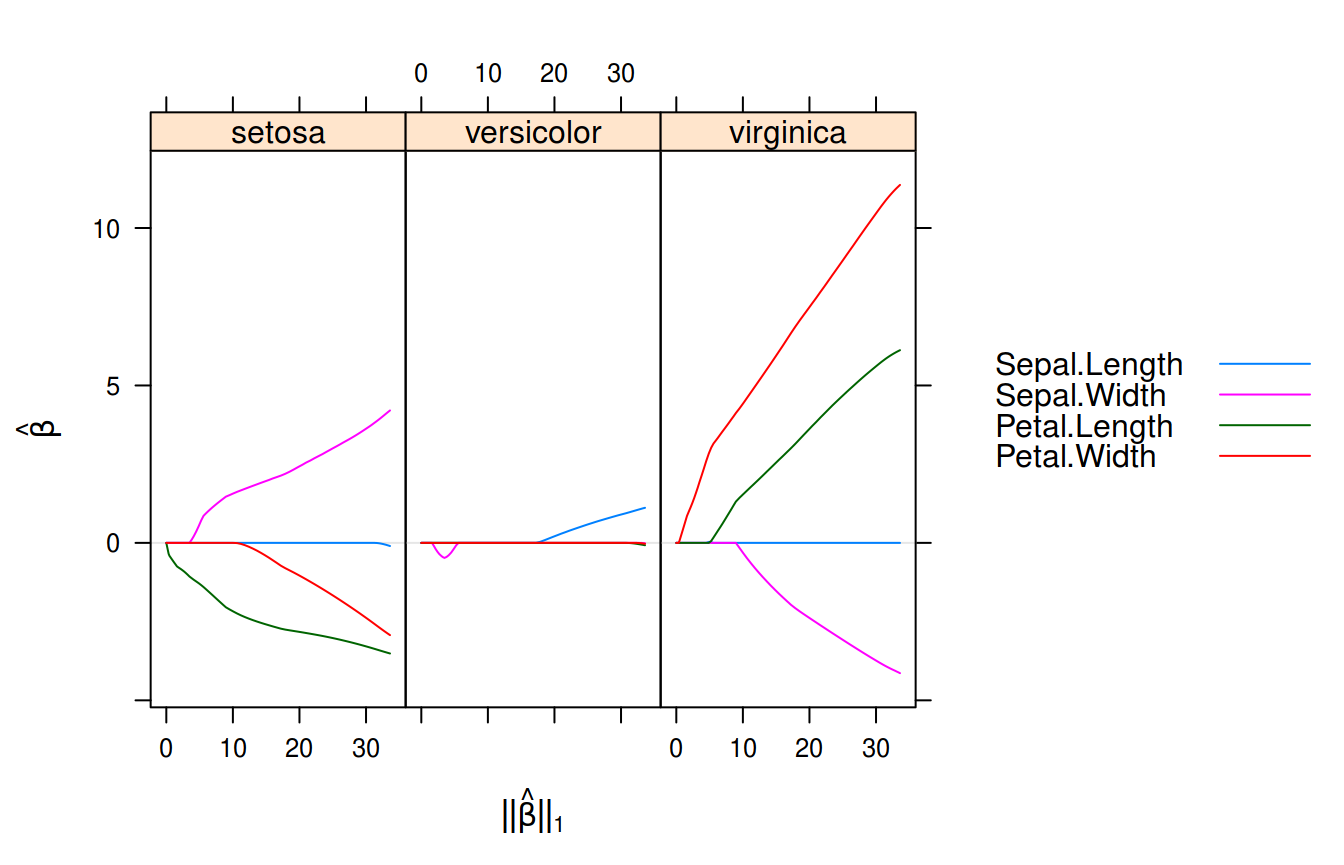
Multinomial logistic regression with sgdnet on the iris data set.

What we see here are the linear predictors for the multinomial model with the \(\ell_1\)-norm along the x-axis. These are always returned on the original scale of the variables even if the argument standardize = TRUE is provided to sgdnet(), which happens to be the default.

Assessing the fit

Now that we have fit our model, we would like to see how well it fits. This is why we left out a testing subset of the data at the start. sgdnet contains a method for predict(), which takes a new set of data and computes predictions for the response based on this.

To predict the class (response) – in this case the species of iris – of the observation, we’ll use the “class” argument.

pred_class <- predict(fit, iris_test[, 1:4], type = "class")

This gives us the class predictions along the entire regularization path. If we had wanted to predict at a specific \(\lambda\), we could have specified it using the s argument in our call to predict().

We’ll now consider the accuracy along the entire path.

acc <- apply(pred_class, 2, function(x) sum(iris_test$Species == x)/length(x))
library(lattice)
xyplot(acc ~ fit$lambda, type = "l",
       xlab = expression(lambda),
       ylab = "Accuracy",
       grid = TRUE)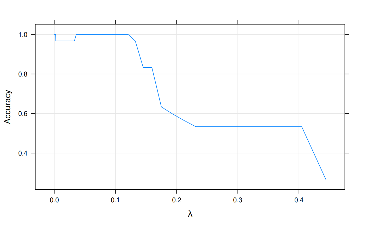

Accuracy in predictions from our model fit to the iris data set.

Of course, the choice of \(\lambda\) cannot be based only on our training data. In any real application we would do best to rely on cross-validation to pick a suitable value.

Acknowledgements

Development on sgdnet begun as a Google Summer of Code project in 2018 with the R Project for Statistical Computing as mentor organization. Michael Weylandt and Toby Dylan Hocking mentored the project.

References

Defazio, Aaron, Francis Bach, and Simon Lacoste-Julien. 2014. “SAGA: A Fast Incremental Gradient Method with Support for Non-Strongly Convex Composite Objectives.” In Advances in Neural Information Processing Systems 27, 2:1646–54. Montreal, Canada: Curran Associates, Inc.

Friedman, Jerome, Trevor Hastie, and Robert Tibshirani. 2010. “Regularization Paths for Generalized Linear Models via Coordinate Descent.” Journal of Statistical Software 33 (1): 1–22. https://doi.org/10.18637/jss.v033.i01.

Johan Larsson