Overview
sgdnet fits generalized linear models of the type
\[ \min_{\beta_0, \beta} \left\{ -\frac1n \mathcal{L}\left(\beta_0,\beta; \mathbf{y}, \mathbf{X}\right) + \lambda \left[(1 - \alpha)||\beta||_2^2 + \alpha||\beta||_1 \right] \right\}, \] where \(\mathcal{L}(\beta_0,\beta; \mathbf{y}, \mathbf{X})\) is the log-likelihood of the model, \(\lambda\) is the regularization strength, and \(\alpha\), is the elastic net mixing parameter (Zou and Hastie 2005), such that \(\alpha = 1\) results in the lasso (Tibshirani 1996) and \(\alpha = 0\) the ridge penalty.
When the lasso penalty is in place, the regularization imposed on the coefficients takes the shape of an octahedron when there are three coefficients.
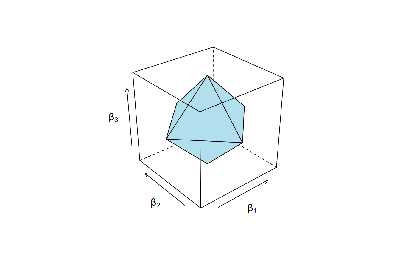
The constraint region for the lasso penalty.
Meanwhile, for ridge regression, this region has the shape of a ball.
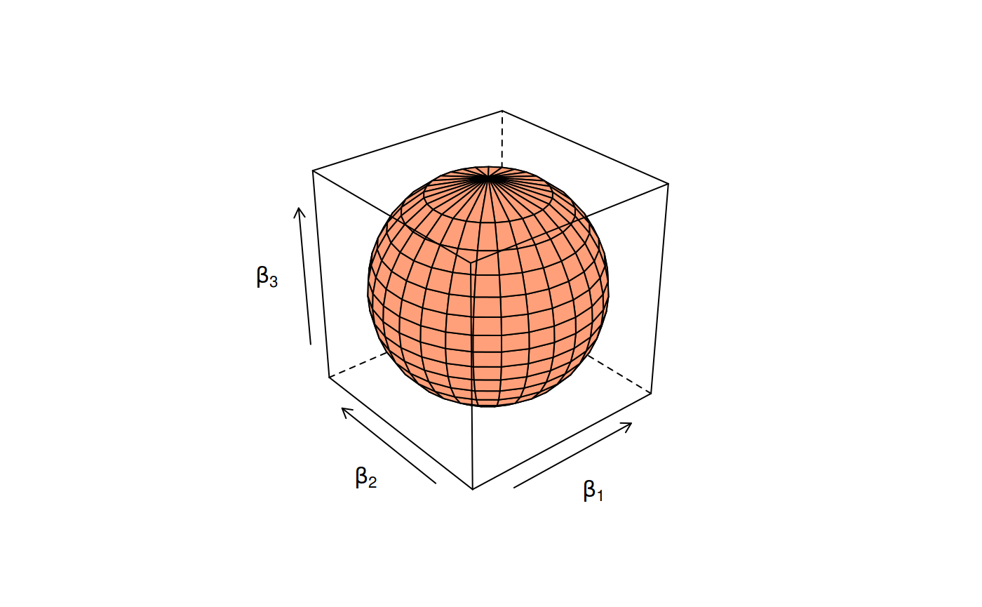
Constraint region for the ridge penalty.
The shape of the elastic net “ball” varies between these two extremes.
We can also use the so-called group lasso penalty on the coefficients. In the following figure, we show the constraint region for the group lasso penalty when \(\beta_1\) and \(\beta_1\) have been grouped.
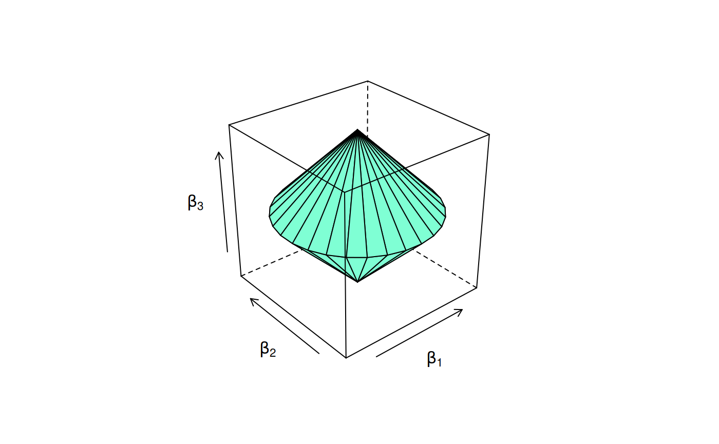
Constraint region for the group lasso penalty.
Gaussian regression
For Gaussian (ordinary least squares) regression, we have the following objective
\[ \min_{\beta_0, \beta} \left\{ \frac{1}{n} \sum_{i=1}^n \left(y_i -\beta_0 - \beta^\intercal \mathbf{x}_i \right)^2 + \lambda \left[(1 - \alpha)||\beta||_2^2 + \alpha||\beta||_1 \right] \right\}. \]
We’ll try to fit this model to the Abalone data set using the regular lasso (alpha = 1) – the default choice. The objective for this data set is to predict the weight of an abalone, a sea snail, using various physical attributes of some 4,177 specimen.
The explicit choice of family is strictly speaking irrelevant here since the Gaussian family is the default choice.
It is worth to mention that the predictors sex and infant are in fact dummy-coded variables from the same categorical predictor. It might make more sense to use a group lasso penalty here and group these predictors so that they are respectively included or excluded together.
Next, we plot the resulting model fits along the regularization path.
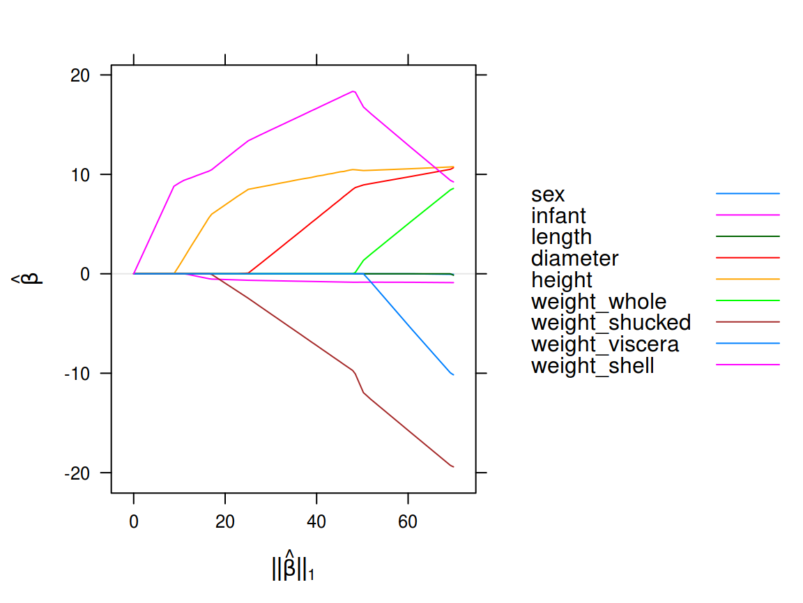
A Gaussian lasso regression fit to the abalone data set
The deviance of this model is the residual sums of squares,
\[ RSS = \sum_{i=1}^{n} \left(y_{i} - \hat\beta_0 - \hat\beta^\intercal \mathbf{x}_{i}\right)^2 \]
which we could retrieve for each fit using deviance(fit_gaussian).
Binomial logistic regression
Binomial logistic regression is a natural solution to binary classification problems. Here, we model the log-likelihood ratio
\[ \log \Bigg[\frac{\text{P}(Y = 1 | X = x)}{\text{P}(Y = 0 | X = x)}\Bigg] = \beta_0 + \beta^\intercal x, \] where \(Y \in \{0, 1\}\). To fit this model, sgdnet uses logistic binomial regression using the logit link, such that
\[ \log \left[ \frac{p(\mathbf{y})}{1-p(\mathbf{y})} \right] = \hat\beta_0 + \sum_{i=1}^n\hat\beta^\intercal \mathbf{x}_i. \]
To fit this model using the elastic net penalty, we minimize the following convex objective:
\[ \min_{\beta_0, \beta} \left\{ -\frac1n \sum_{i=1}^n \bigg[y_i (\beta_0 + \beta^\intercal x_i) - \log\Big(1 + e^{\beta_0 + \beta^\intercal x_i}\Big)\bigg] + \lambda \left[(1 - \alpha)||\beta||_2^2 + \alpha||\beta||_1 \right] \right\}. \]
To illustate fitting the binomial logistic model with sgdnet, we’ll take a look at the Heart Disease data set. In this set, we try to predict heart disease using a variety of clinical assessments such as blood pressure, heart rate, and electrocardiography results.
This time, we’ll employ ridge regression instead, setting \(\alpha = 0\)
binomial_fit <- sgdnet(heart$x, heart$y, family = "binomial", alpha = 0)
plot(binomial_fit)
plot(binomial_fit, xvar = "lambda")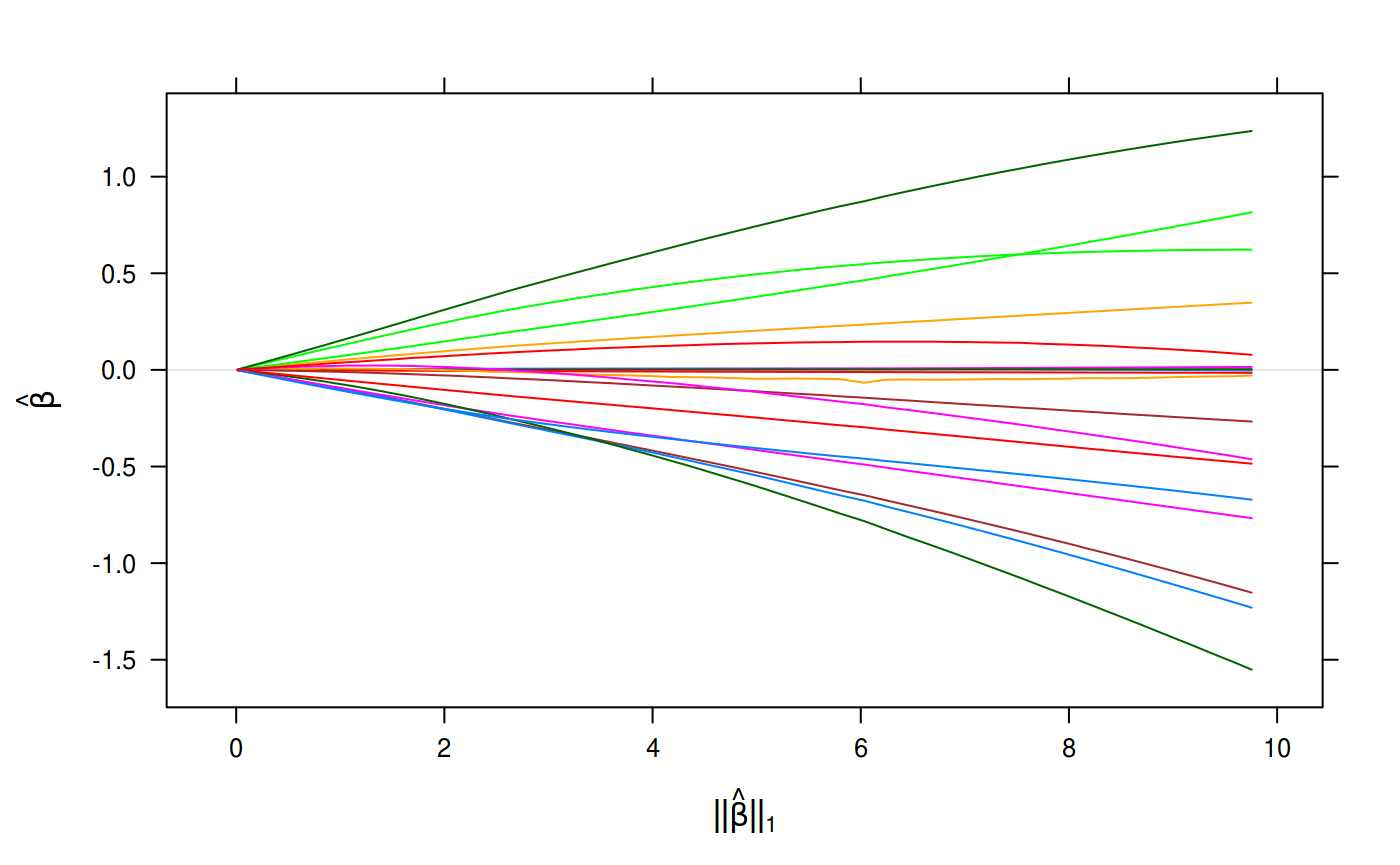
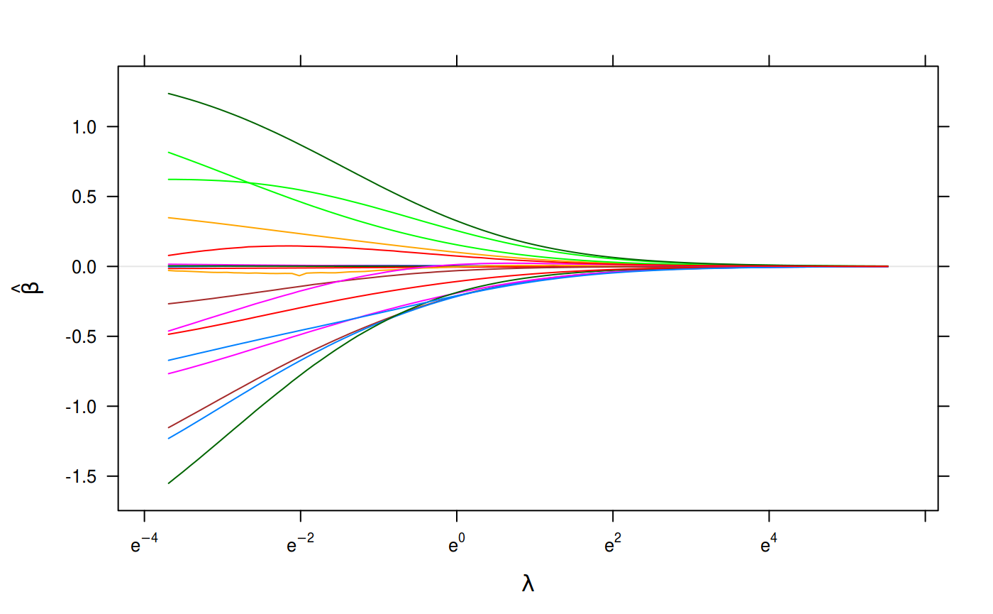
Binomial Regression on the Heart Disease Data Set.
Multinomial logistic regression
Multinomial logistic regression is concerned with classifying categorical outcomes using the multinomial likelihood. Here we use the loglinear representation
\[ \text{Pr}(Y_i = c) = \frac{e^{\beta_{0_c}+\beta_c^\intercal \mathbf{x}_i}}{\sum_{k = 1}^K{e^{\beta_{0_k}+\beta_k^\intercal \mathbf{x}_i}}}, \]
which is overspecified in its non-regularized form, lacking a unique solution since we can shift the coefficients by a constant and still yield the same class probabilities. However, as in glmnet (Friedman, Hastie, and Tibshirani 2010) – which much of this packages functionality is modeled after – we rely on the regularization to take are of this (Hastie, Tibshirani, and Wainwright 2015, 36–37). This works because, with the added regularization, the solutions are no longer indifferent to a shift in the coefficients.
The objective for the multinomial logistic regression is then
\[ \min_{\{\beta_{0_k}, \beta_k\}_1^K} \left\{ -\frac1n \sum_{i=1}^n \left[\sum_{k=1}^K y_{i_k} (\beta_{0_k}+\beta_k^\intercal \mathbf{x}_i) - \log \sum_{k=1}^K e^{\beta_{0_k}+\beta_k^\intercal \mathbf{x}_i}\right] + \lambda \left[(1 - \alpha)||\beta||_F ^2 + \alpha\sum_{j=1}^p||\beta_j||_q \right] \right\}. \]
where \(q = 1\) invokes the standard lasso and \(q = 2\) for the group lasso penalty.
The example for this model family comes from the Wine data set where we attempt to classify a number of wines from Italy using the results of chemical analysis.
We will use the elastic net penalty this time, setting it (arbitrarily) at 0.8.
multinomial_fit <- sgdnet(wine$x, wine$y, family = "multinomial")
plot(multinomial_fit, layout = c(3, 1))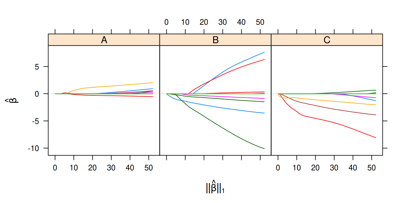
Multinomial logistic regression on the wine data set.
Multivariate gaussian regression
Multivariate gaussian models, fit using family = "mgaussian" in the call to sgdnet(), are useful when there are several correlated and numeric responses. The objective for this model is to minimize
\[ \frac{1}{2n} ||\mathbf{Y} -\mathbf{B}_0\mathbf{1} - \mathbf{B} \mathbf{X}||^2_F + \lambda \left((1 - \alpha)/2||\mathbf{B}||_F^2 + \alpha ||\mathbf{B}||_{12}\right), \] where \(\mathbf{Y}\) is a matrix of responses, \(\mathbf{B}\) is a matrix of coefficients, and \(\mathbf{1}\) is a matrix of all ones.
\(\alpha ||\mathbf{B}||_{12}\) in the penalty-part of the objective is the group lasso, which enables feature selection such that each column of coefficients in \(\mathbf{B}\) each either in or out simultaneously. The proximal operator for the group lasso is given by
\[ \beta_j \leftarrow \left( 1 - \frac{\gamma\lambda\alpha}{||\beta_j||_2} \right)_+\beta_j, \] where the subscript \(+\) indicates the positive part of \((\cdot)\) and \(\gamma\) is the step size. \(\beta\) is the vector of coefficients corresponding to response \(j\).
Our example data set for this model comes in the shape of student performance data. We have two responses indicating the final grade of a student in maths and portugese respectively.
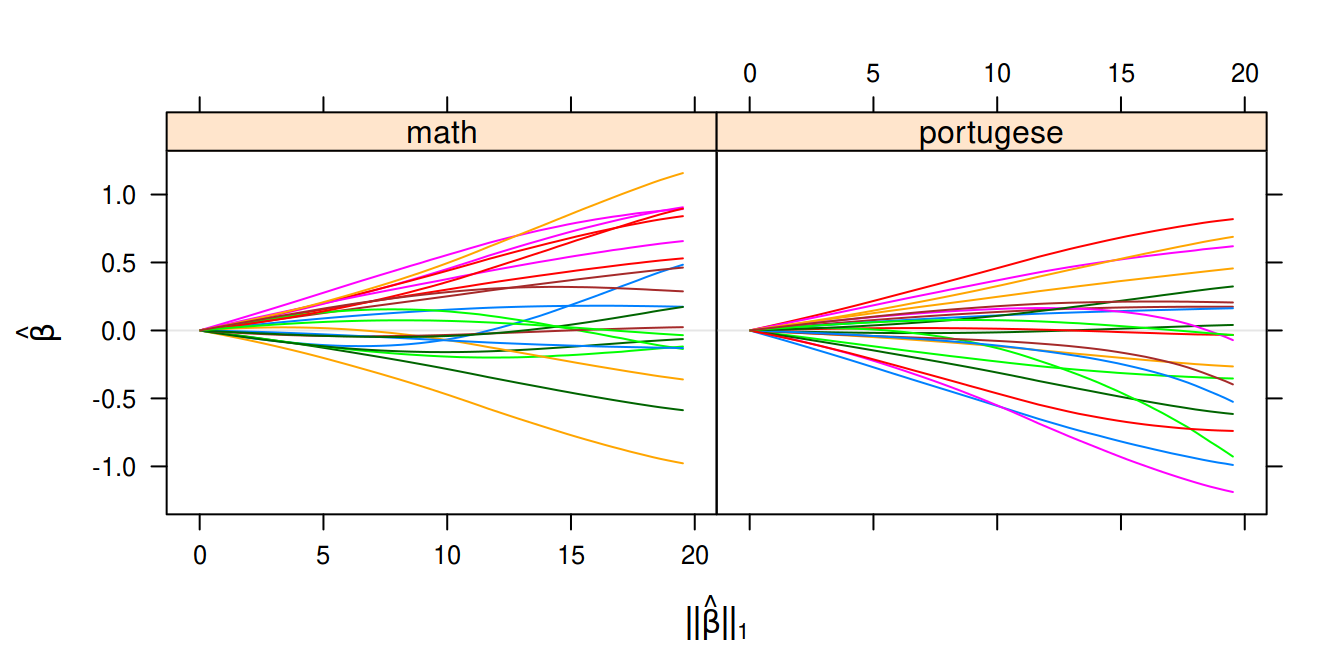
Multivariate Gaussian regression on the Student Performance Data Set.
This family has an additional parameter, standardize.response, which enables us to standardize the response as well but, given that the responses are already on the same scale, we refrain.
References
Friedman, Jerome, Trevor Hastie, and Robert Tibshirani. 2010. “Regularization Paths for Generalized Linear Models via Coordinate Descent.” Journal of Statistical Software 33 (1): 1–22. https://doi.org/10.18637/jss.v033.i01.
Hastie, Trevor, Robert Tibshirani, and Martin Wainwright. 2015. Statistical Learning with Sparsity: The Lasso and Generalizations. 1 edition. Boca Raton: Chapman and Hall/CRC.
Tibshirani, Robert. 1996. “Regression Shrinkage and Selection via the Lasso.” Journal of the Royal Statistical Society. Series B (Methodological) 58 (1): 267–88.
Zou, Hui, and Trevor Hastie. 2005. “Regularization and Variable Selection via the Elastic Net.” Journal of the Royal Statistical Society. Series B (Statistical Methodology) 67 (2): 301–20.