Motivation
eulerr generates area-proportional euler diagrams that display set relationships (intersections, unions, and disjoints) with circles, ellipses, or axis-aligned rectangles and squares. Euler diagrams are Venn diagrams without the requirement that all set interactions be present (whether they are empty or not). That is, depending on input, eulerr will sometimes produce Venn diagrams but sometimes not.
R features several packages that produce Euler diagrams; some of the more prominent ones (on CRAN) are
The last of these (venneuler) was the primary inspiration for this package, along with the refinements that Fredrickson has presented on his blog and made available in his javascript venn.js. eulerAPE, which was the first program to uses ellipses instead of circles, has also been instrumental in the design of eulerr. The downside to eulerAPE is that it only handles three sets that all need to intersect.
venneuler, on the other hand, will take any number of sets (in theory), yet has been known to produce imperfect solutions for set configurations that have perfect such. And unlike eulerAPE, it is restricted to circles (as is venn.js).
Enter eulerr
eulerr is based on the improvements to venneuler that Ben Fredrickson introduced with venn.js but has been programmed from scratch, uses different optimizers, and returns statistics featured in venneuler and eulerAPE as well as allows a range of different inputs and conditioning on additional variables. Moreover, it can model set relationships with ellipses for any number of sets involved.
Input
At the time of writing, it is possible to provide input to eulerr as either
- a named numeric vector with set combinations as disjoint set
combinations or unions (depending on how the argument
typeis set ineuler()), - a matrix or data frame of logicals with columns representing sets and rows the set relationships for each observation,
- a list of sample spaces, or
- a table.
library(eulerr)

# Input in the form of a named numeric vector
fit1 <- euler(c(
  "A" = 25,
  "B" = 5,
  "C" = 5,
  "A&B" = 5,
  "A&C" = 5,
  "B&C" = 3,
  "A&B&C" = 3
))

# Input as a matrix of logicals
set.seed(1)
mat <- cbind(
  A = sample(c(TRUE, TRUE, FALSE), 50, TRUE),
  B = sample(c(TRUE, FALSE), 50, TRUE),
  C = sample(c(TRUE, FALSE, FALSE, FALSE), 50, TRUE)
)
fit2 <- euler(mat)
We inspect our results by printing the eulerr object
fit2
#>       original fitted residuals regionError
#> A           13     13         0       0.008
#> B            4      4         0       0.002
#> C            0      0         0       0.000
#> A&B         17     17         0       0.010
#> A&C          5      5         0       0.003
#> B&C          1      0         1       0.024
#> A&B&C        2      2         0       0.001
#>
#> diagError: 0.024
#> stress:    0.002
or directly access and plot the residuals.
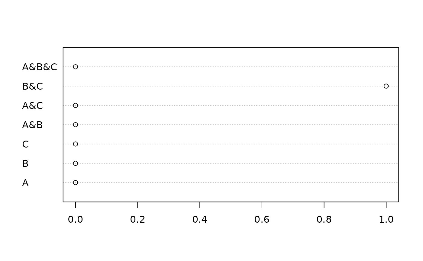
Residuals for the fit diagram.
We can also use eulerr’s built in
error_plot() function to diagnose the fit.
{r error-plot, fig.cap = "A plot from `error_plot()`."} error_plot(fit2)
This shows us that the intersection is somewhat overrepresented in . Given that these residuals are on the scale of the original values, however, the residuals are arguably of little concern.
As an alternative, we could plot the circles in another program by retrieving their coordinates and radii.
coef(fit2)
#>     type       h         k     a     b phi width height side
#> A circle -0.4587 2.220e-16 3.432 3.432   0   NaN    NaN  NaN
#> B circle  1.1847 1.110e-16 2.706 2.706   0   NaN    NaN  NaN
#> C circle -1.4189 1.685e+00 1.493 1.493   0   NaN    NaN  NaN
Goodness-of-fit
To tell if we can trust our solution, we use two goodness-of-fit measures: the stress statistic from venneuler (Wilkinson 2012),
where is an ordinary least squares estimate from the regression of the fitted areas on the original areas that is being explored during optimization,
and the diagError statistic from eulerAPE (Micallef and Rodgers 2014):
In our example, the diagError is and our stress is 0.002, suggesting that the fit is accurate.
We can now be confident that eulerr provides a reasonable
representation of our input using circles. Were it otherwise, we might
try a different shape via the shape argument —
"ellipse" is the most expressive choice, but axis-aligned
"rectangle" and "square" fits are also
available. (Wilkinson 2012) features a
difficult combination that ellipses manage to fit with a reasonably
small error; with eulerr, however, we can get rid of
that error entirely.
wilkinson2012 <- c(
  A = 4,
  B = 6,
  C = 3,
  D = 2,
  E = 7,
  F = 3,
  "A&B" = 2,
  "A&F" = 2,
  "B&C" = 2,
  "B&D" = 1,
  "B&F" = 2,
  "C&D" = 1,
  "D&E" = 1,
  "E&F" = 1,
  "A&B&F" = 1,
  "B&C&D" = 1
)
fit3 <- euler(wilkinson2012, shape = "ellipse")
plot(fit3)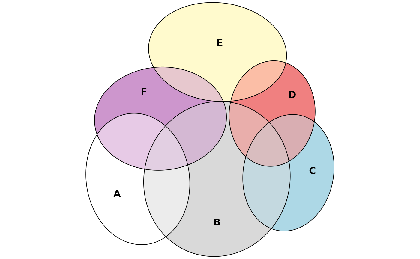
A difficult combination from Wilkinson 2012.
If we still lack a good fit after having tried ellipses, we would do best to stop here and look for another way to visualize our data. (I suggest the excellent UpSetR package.)
Visualization
No we get to the fun part: plotting our diagram. This is easy, as well as highly customizable, with eulerr. The default parameters can easily be adjusted to suit anybody’s needs.
plot(fit2)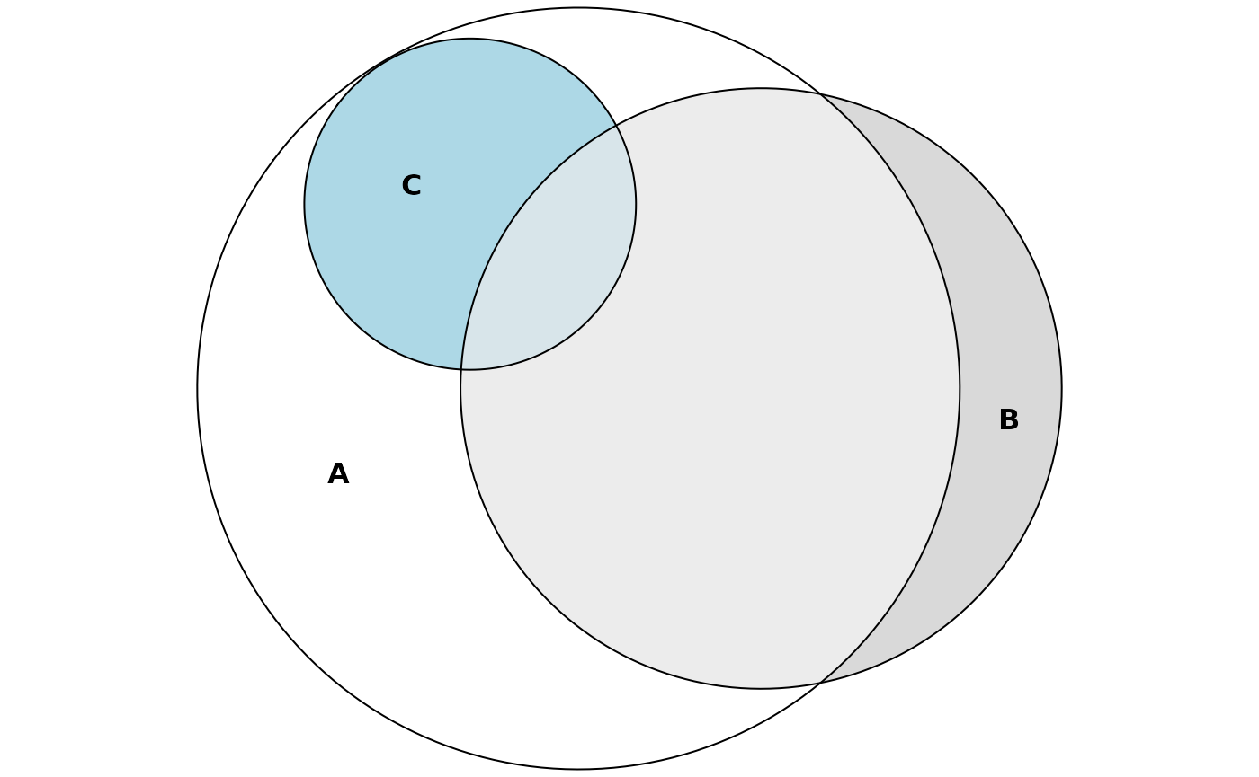
Customizing Euler plots is a breeze in eulerr.
# Switch to squares for the same set combination, customizing borders,
# labels, and quantities. The `shape` argument also accepts `"ellipse"`
# and `"rectangle"`.
plot(
  euler(mat, shape = "square"),
  quantities = TRUE,
  fill = "transparent",
  lty = 1:3,
  labels = list(font = 4)
)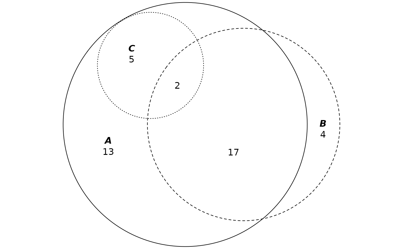
Customizing Euler plots is a breeze in eulerr.
Plotting is provided through a custom plotting method built on top of the excellent facilities made available by the core R package grid. eulerr’s default color palette is chosen to be color deficiency-friendly.
Acknowledgements
eulerr would not be possible without Ben Fredrickson’s work on venn.js or Leland Wilkinson’s venneuler.