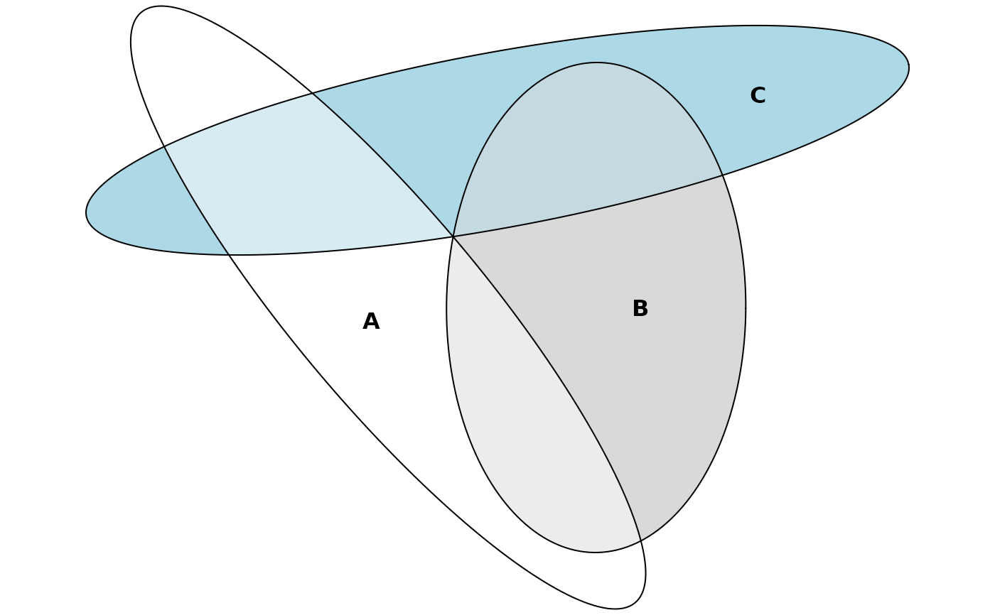
Fit Euler diagrams (a generalization of Venn diagrams) using numerical optimization to find exact or approximate solutions to a specification of set relationships. The shape of the diagram may be a circle, an ellipse, an axis-aligned rectangle, or an axis-aligned square.
Usage
euler(combinations, ...)

# Default S3 method
euler(
  combinations,
  input = c("disjoint", "union"),
  transform = identity,
  shape = c("circle", "ellipse", "rectangle", "square", "rotated_rectangle"),
  loss = c("sum_squared", "sum_absolute", "sum_absolute_region_error",
    "sum_squared_region_error", "max_absolute", "max_squared", "root_mean_squared",
    "stress", "diag_error", "log_sum_absolute", "smooth_sum_absolute",
    "smooth_sum_absolute_region_error", "smooth_max_absolute", "smooth_max_squared",
    "smooth_diag_error", "smooth_log_sum_absolute"),
  loss_aggregator = NULL,
  complement = NULL,
  control = list(),
  ...
)

# S3 method for class 'data.frame'
euler(
  combinations,
  weights = NULL,
  by = NULL,
  sep = "_",
  factor_names = TRUE,
  ...
)

# S3 method for class 'matrix'
euler(combinations, ...)

# S3 method for class 'table'
euler(combinations, ...)

# S3 method for class 'list'
euler(combinations, ...)
Arguments
- combinations
set relationships as a named numeric vector, matrix, or data.frame (see methods (by class))
- ...
arguments passed down to other methods
- input
type of input: disjoint identities (
'disjoint') or unions ('union').- transform
a function applied to the areas of the disjoint (exclusive) regions before fitting. The default,
base::identity(), leaves the areas untouched. A monotone transform such asbase::log1p()can keep small regions legible when set sizes span several orders of magnitude. The transform is applied to the exclusive regions because those are the additive atoms the diagram fits to; as a consequence the area of a whole set or union no longer equalstransform()of its size, only the individual visible regions carry the transformed scale. The function must return a non-negative, finite value for each region (and forcomplement, when given). Has no effect onvenn()diagrams, whose geometry is fixed.- shape
geometric shape used in the diagram: one of
"circle","ellipse","rectangle","square", or"rotated_rectangle". The rotated rectangle is fit with a derivative-free optimizer and is also the only shape able to draw a true four-set Venn diagram (seevenn()).- loss
type of loss to minimize over. The default,
"sum_squared", minimizes the sum of squared errors. The available options mirror the loss functions exposed by theeunoiaRust crate that powers the optimizer:"sum_squared": normalized sum of squared errors (default)."sum_absolute": normalized sum of absolute errors."sum_absolute_region_error": normalized sum of absolute region errors."sum_squared_region_error": normalized sum of squared region errors."max_absolute": normalized maximum absolute error."max_squared": normalized maximum squared error."root_mean_squared": normalized root-mean-squared error."stress": venneuler-style stress."diag_error": eulerAPE-stylediagError."log_sum_absolute": sum of absolute errors onlog1p-transformed areas, which stops large regions from dominating the fit."smooth_sum_absolute","smooth_sum_absolute_region_error","smooth_max_absolute","smooth_max_squared","smooth_diag_error","smooth_log_sum_absolute"— gradient-friendly (Huber) surrogates of the corresponding non-smooth losses, controlled bycontrol$loss_eps.
- loss_aggregator
deprecated; use
lossdirectly instead. Pre-1.0 code that combinedloss("square"/"abs"/"region") withloss_aggregator("sum"/"max") still works but emits a warning; the combination is mapped to the equivalent newlossvalue.- complement
an optional single non-negative number giving the area of the complement, that is, the universe outside every named set. When supplied, the fitter jointly optimizes a containing rectangle together with the diagram shapes so that the area of the rectangle minus the union of (clipped) shapes matches
complement. This is the classical "everything not in any set" region; seeplot.euler()for how it is rendered. Defaults toNULL(no container; classical shape-only fit). Not supported forvenn().- control
a list of control parameters.
extraopt: should the global-search fallback optimizer (CMA-ES) kick in when the primary optimizer'sdiagErrorexceedsextraopt_threshold? The default isTRUEfor three-set ellipse fits andFALSEotherwise.extraopt_threshold: threshold, in terms ofdiagError, for when the CMA-ES fallback kicks in. A value of 0 means it will kick in for an* error; a value of 1 means it will never kick in. Default0.001.tolerance: convergence tolerance passed to the underlying solver. Tighter values give more accurate fits at higher cost. Default1e-8.max_sets: maximum number of sets the underlying engine will accept. Defaults toNULL, which uses the engine's built-in default of 32. Region masks are stored in a bitset, so values may be raised up to 63 (the absolute hard cap). Going higher is rarely useful in practice since fully-overlapping diagrams have2^n - 1regions.n_threads: number of threads used to fan out the optimizer's restart loop. A positive integer pins a private thread pool of that size, whileNULLuses all available cores. This is purely a wall-time knob: the fitted diagram is identical regardless of the thread count. The default uses half of the available logical cores (but a single thread underR CMD check, to respect CRAN's two-core policy). It can be overridden globally with theeulerr.n_threadsoption or theEULERR_NUM_THREADSenvironment variable, and otherwise honors R's conventionalmc.coresoption (orMC_CORESenvironment variable).optimizer: the final-layout optimizer. The default,"auto", lets the engine pick a sensible optimizer for the chosen shape and loss. To force a particular one, use any of"levenberg_marquardt","lbfgs","nelder_mead","mads"(mesh-adaptive direct search, derivative-free and well suited to non-smooth losses),"cma_es","cma_es_lm","trf", or"cma_es_trf".n_restarts: number of full-pipeline restarts; the lowest-loss result is kept. Higher values improve the chance of finding the global optimum at proportionally higher cost.NULL(the default) lets the engine choose (10, automatically reduced for small smooth-loss fits).loss_eps: smoothing parameter for the"smooth_*"losses; pick roughly 1% of the typical residual magnitude. Smaller values track the non-smooth loss more closely but give noisier gradients. Default0.01.
- weights
a numeric vector of weights of the same length as the number of rows in
combinations.- by
a factor or character matrix to be used in
base::by()to split the data.frame or matrix of set combinations- sep
a character to use to separate the dummy-coded factors if there are factor or character vectors in 'combinations'.
- factor_names
whether to include factor names when constructing dummy codes
Value
A list object of class 'euler' with the following parameters.
- shapes
a data frame of fitted shape parameters. One row per set with a
typecolumn (one of"circle","ellipse","rectangle","square","rotated_rectangle"), the center coordinateshandk, and the shape-specific columns:a,b,phifor ellipses/circles;widthandheightfor rectangles;side(plus mirroredwidth/height) for squares;width,height, andphi(rotation, in radians) for rotated rectangles. Columns that don't apply to the chosen shape areNA.- ellipses
for
shape = "circle"andshape = "ellipse"fits, the legacy 5-column data frame ofh,k,a,b,phi. This slot is deprecated in favour ofshapesand is not populated for rectangle/square fits.- original.values
set relationships in the input
- fitted.values
set relationships in the solution
- residuals
residuals
- regionError
the difference in percentage points between each disjoint subset in the input and the respective area in the output
- diagError
the largest
regionError- stress
normalized residual sums of squares
Details
If the input is a matrix or data frame and argument by is specified,
the function returns a list of euler diagrams.
The function minimizes the residual sums of squares,
$$
\sum_{i=1}^n (A_i - \omega_i)^2,
$$
by default, where \(\omega_i\) the size of the ith disjoint subset, and
\(A_i\) the corresponding area in the diagram, that is, the unique
contribution to the total area from this overlap. The loss function
can, however, be controlled via the loss argument.
euler() also returns stress (from venneuler), as well as
diagError, and regionError from eulerAPE.
The stress statistic is computed as
$$ \frac{\sum_{i=1}^n (A_i - \beta\omega_i)^2}{\sum_{i=1}^n A_i^2}, $$ where $$ \beta = \sum_{i=1}^n A_i\omega_i / \sum_{i=1}^n \omega_i^2. $$
regionError is computed as
$$ \left| \frac{A_i}{\sum_{i=1}^n A_i} - \frac{\omega_i}{\sum_{i=1}^n \omega_i}\right|. $$
diagError is simply the maximum of regionError.
Methods (by class)
euler(default): a named numeric vector, with combinations separated by an ampersand, for instanceA&B = 10. Missing combinations are treated as being 0.euler(data.frame): adata.frameof logicals, binary integers, or factors.euler(matrix): a matrix that can be converted to a data.frame of logicals (as in the description above) viabase::as.data.frame.matrix().euler(table): A table withmax(dim(x)) < 3.euler(list): a list of vectors, each vector giving the contents of that set (with no duplicates). Vectors in the list must be named.
References
Wilkinson L. Exact and Approximate Area-Proportional Circular Venn and Euler Diagrams. IEEE Transactions on Visualization and Computer Graphics (Internet). 2012 Feb (cited 2016 Apr 9);18(2):321-31. Available from: doi:10.1109/TVCG.2011.56
Micallef L, Rodgers P. eulerAPE: Drawing Area-Proportional 3-Venn Diagrams Using Ellipses. PLOS ONE (Internet). 2014 Jul (cited 2016 Dec 10);9(7):e101717. Available from: doi:10.1371/journal.pone.0101717
Examples
# Fit a diagram with circles
combo <- c(A = 2, B = 2, C = 2, "A&B" = 1, "A&C" = 1, "B&C" = 1)
fit1 <- euler(combo)
# Investigate the fit
fit1
#> original fitted residuals regionError
#> A 2 2.076 -0.076 0.021
#> B 2 2.076 -0.076 0.021
#> C 2 2.076 -0.076 0.021
#> A&B 1 0.605 0.395 0.040
#> A&C 1 0.605 0.395 0.040
#> B&C 1 0.605 0.395 0.040
#> A&B&C 0 0.494 -0.494 0.058
#>
#> diagError: 0.058
#> stress: 0.049
# Refit using ellipses instead
fit2 <- euler(combo, shape = "ellipse")
# Investigate the fit again (which is now exact)
fit2
#> original fitted residuals regionError
#> A 2 2 0 0
#> B 2 2 0 0
#> C 2 2 0 0
#> A&B 1 1 0 0
#> A&C 1 1 0 0
#> B&C 1 1 0 0
#> A&B&C 0 0 0 0
#>
#> diagError: 0
#> stress: 0
# Plot it
plot(fit2)
 # A set with no perfect solution
euler(c(
"a" = 3491, "b" = 3409, "c" = 3503,
"a&b" = 120, "a&c" = 114, "b&c" = 132,
"a&b&c" = 50
))
#> original fitted residuals regionError
#> a 3491 3491 0 0.001
#> b 3409 3409 0 0.001
#> c 3503 3503 0 0.002
#> a&b 120 120 0 0.000
#> a&c 114 114 0 0.000
#> b&c 132 132 0 0.000
#> a&b&c 50 0 50 0.005
#>
#> diagError: 0.005
#> stress: 0
# Using grouping via the 'by' argument through the data.frame method
euler(fruits, by = list(sex, age))
#> female.adult
#> original fitted residuals regionError
#> banana 1 0.937 0.063 0.009
#> apple 2 1.968 0.032 0.009
#> orange 2 1.974 0.026 0.009
#> banana&apple 4 4.028 -0.028 0.010
#> banana&orange 0 0.268 -0.268 0.024
#> apple&orange 0 0.260 -0.260 0.023
#> banana&apple&orange 2 1.961 0.039 0.010
#>
#> diagError: 0.024
#> stress: 0.005
#> ------------------------------------------------------------
#> male.child
#> original fitted residuals regionError
#> banana 3 2.994 0.006 0.003
#> apple 1 0.982 0.018 0.002
#> orange 1 0.981 0.019 0.002
#> banana&apple 10 10.004 -0.004 0.007
#> banana&orange 0 0.137 -0.137 0.008
#> apple&orange 0 0.144 -0.144 0.008
#> banana&apple&orange 3 2.993 0.007 0.003
#>
#> diagError: 0.008
#> stress: 0
#> ------------------------------------------------------------
#> male.adult
#> original fitted residuals regionError
#> banana 3 3.000 0.000 0.000
#> apple 2 2.003 -0.003 0.000
#> orange 0 0.016 -0.016 0.001
#> banana&apple 10 10.000 0.000 0.001
#> apple&orange 1 0.996 0.004 0.000
#> banana&apple&orange 1 1.002 -0.002 0.000
#>
#> diagError: 0.001
#> stress: 0
#> ------------------------------------------------------------
#> female.child
#> original fitted residuals regionError
#> banana 4 4 0 0
#> apple 0 0 0 0
#> orange 1 1 0 0
#> banana&apple 4 4 0 0
#> banana&orange 1 1 0 0
#> banana&apple&orange 2 2 0 0
#>
#> diagError: 0
#> stress: 0
# Using the matrix method
euler(organisms)
#> original fitted residuals regionError
#> animal 0 0.582 -0.582 0.086
#> mammal 0 0.302 -0.302 0.044
#> plant 0 0.210 -0.210 0.031
#> sea 0 0.430 -0.430 0.063
#> spiny 0 0.166 -0.166 0.025
#> animal&mammal 2 1.817 0.183 0.018
#> animal&sea 1 0.612 0.388 0.053
#> animal&spiny 0 0.215 -0.215 0.032
#> mammal&sea 1 0.000 1.000 0.143
#> plant&sea 1 0.868 0.132 0.015
#> plant&spiny 1 0.000 1.000 0.143
#> sea&spiny 0 0.176 -0.176 0.026
#> animal&mammal&sea 0 0.268 -0.268 0.040
#> animal&mammal&spiny 0 0.061 -0.061 0.009
#> animal&plant&sea 0 0.119 -0.119 0.018
#> animal&sea&spiny 1 0.715 0.285 0.037
#> plant&sea&spiny 0 0.016 -0.016 0.002
#> animal&mammal&sea&spiny 0 0.177 -0.177 0.026
#> animal&plant&sea&spiny 0 0.043 -0.043 0.006
#>
#> diagError: 0.143
#> stress: 0.352
# Using weights
euler(organisms, weights = c(10, 20, 5, 4, 8, 9, 2))
#> original fitted residuals regionError
#> animal 0 1.829 -1.829 0.033
#> mammal 0 3.612 -3.612 0.065
#> plant 0 0.769 -0.769 0.014
#> sea 0 1.900 -1.900 0.034
#> spiny 0 0.374 -0.374 0.007
#> animal&mammal 30 29.532 0.468 0.018
#> animal&sea 4 0.000 4.000 0.069
#> mammal&plant 0 0.859 -0.859 0.016
#> mammal&sea 8 3.072 4.928 0.082
#> plant&sea 2 0.000 2.000 0.034
#> plant&spiny 9 9.004 -0.004 0.008
#> animal&mammal&plant 0 0.487 -0.487 0.009
#> animal&mammal&sea 0 2.216 -2.216 0.040
#> animal&sea&spiny 5 0.000 5.000 0.086
#> mammal&plant&sea 0 0.000 0.000 0.000
#> mammal&plant&spiny 0 1.513 -1.513 0.027
#>
#> diagError: 0.086
#> stress: 0.09
# The table method
euler(pain, factor_names = FALSE)
#> original fitted residuals regionError
#> widespread 204 204.002 -0.002 0
#> regional 229 229.002 -0.002 0
#> male 48 48.032 -0.032 0
#> widespread&male 78 77.984 0.016 0
#> regional&male 143 142.992 0.008 0
#> widespread®ional&male 0 0.247 -0.247 0
#>
#> diagError: 0
#> stress: 0
# A euler diagram from a list of sample spaces (the list method)
euler(plants[c("erigenia", "solanum", "cynodon")])
#> original fitted residuals regionError
#> erigenia 0 0 0 0
#> solanum 16 16 0 0
#> cynodon 1 1 0 0
#> erigenia&solanum 2 2 0 0
#> solanum&cynodon 25 25 0 0
#> erigenia&solanum&cynodon 20 20 0 0
#>
#> diagError: 0
#> stress: 0
# A set with no perfect solution
euler(c(
"a" = 3491, "b" = 3409, "c" = 3503,
"a&b" = 120, "a&c" = 114, "b&c" = 132,
"a&b&c" = 50
))
#> original fitted residuals regionError
#> a 3491 3491 0 0.001
#> b 3409 3409 0 0.001
#> c 3503 3503 0 0.002
#> a&b 120 120 0 0.000
#> a&c 114 114 0 0.000
#> b&c 132 132 0 0.000
#> a&b&c 50 0 50 0.005
#>
#> diagError: 0.005
#> stress: 0
# Using grouping via the 'by' argument through the data.frame method
euler(fruits, by = list(sex, age))
#> female.adult
#> original fitted residuals regionError
#> banana 1 0.937 0.063 0.009
#> apple 2 1.968 0.032 0.009
#> orange 2 1.974 0.026 0.009
#> banana&apple 4 4.028 -0.028 0.010
#> banana&orange 0 0.268 -0.268 0.024
#> apple&orange 0 0.260 -0.260 0.023
#> banana&apple&orange 2 1.961 0.039 0.010
#>
#> diagError: 0.024
#> stress: 0.005
#> ------------------------------------------------------------
#> male.child
#> original fitted residuals regionError
#> banana 3 2.994 0.006 0.003
#> apple 1 0.982 0.018 0.002
#> orange 1 0.981 0.019 0.002
#> banana&apple 10 10.004 -0.004 0.007
#> banana&orange 0 0.137 -0.137 0.008
#> apple&orange 0 0.144 -0.144 0.008
#> banana&apple&orange 3 2.993 0.007 0.003
#>
#> diagError: 0.008
#> stress: 0
#> ------------------------------------------------------------
#> male.adult
#> original fitted residuals regionError
#> banana 3 3.000 0.000 0.000
#> apple 2 2.003 -0.003 0.000
#> orange 0 0.016 -0.016 0.001
#> banana&apple 10 10.000 0.000 0.001
#> apple&orange 1 0.996 0.004 0.000
#> banana&apple&orange 1 1.002 -0.002 0.000
#>
#> diagError: 0.001
#> stress: 0
#> ------------------------------------------------------------
#> female.child
#> original fitted residuals regionError
#> banana 4 4 0 0
#> apple 0 0 0 0
#> orange 1 1 0 0
#> banana&apple 4 4 0 0
#> banana&orange 1 1 0 0
#> banana&apple&orange 2 2 0 0
#>
#> diagError: 0
#> stress: 0
# Using the matrix method
euler(organisms)
#> original fitted residuals regionError
#> animal 0 0.582 -0.582 0.086
#> mammal 0 0.302 -0.302 0.044
#> plant 0 0.210 -0.210 0.031
#> sea 0 0.430 -0.430 0.063
#> spiny 0 0.166 -0.166 0.025
#> animal&mammal 2 1.817 0.183 0.018
#> animal&sea 1 0.612 0.388 0.053
#> animal&spiny 0 0.215 -0.215 0.032
#> mammal&sea 1 0.000 1.000 0.143
#> plant&sea 1 0.868 0.132 0.015
#> plant&spiny 1 0.000 1.000 0.143
#> sea&spiny 0 0.176 -0.176 0.026
#> animal&mammal&sea 0 0.268 -0.268 0.040
#> animal&mammal&spiny 0 0.061 -0.061 0.009
#> animal&plant&sea 0 0.119 -0.119 0.018
#> animal&sea&spiny 1 0.715 0.285 0.037
#> plant&sea&spiny 0 0.016 -0.016 0.002
#> animal&mammal&sea&spiny 0 0.177 -0.177 0.026
#> animal&plant&sea&spiny 0 0.043 -0.043 0.006
#>
#> diagError: 0.143
#> stress: 0.352
# Using weights
euler(organisms, weights = c(10, 20, 5, 4, 8, 9, 2))
#> original fitted residuals regionError
#> animal 0 1.829 -1.829 0.033
#> mammal 0 3.612 -3.612 0.065
#> plant 0 0.769 -0.769 0.014
#> sea 0 1.900 -1.900 0.034
#> spiny 0 0.374 -0.374 0.007
#> animal&mammal 30 29.532 0.468 0.018
#> animal&sea 4 0.000 4.000 0.069
#> mammal&plant 0 0.859 -0.859 0.016
#> mammal&sea 8 3.072 4.928 0.082
#> plant&sea 2 0.000 2.000 0.034
#> plant&spiny 9 9.004 -0.004 0.008
#> animal&mammal&plant 0 0.487 -0.487 0.009
#> animal&mammal&sea 0 2.216 -2.216 0.040
#> animal&sea&spiny 5 0.000 5.000 0.086
#> mammal&plant&sea 0 0.000 0.000 0.000
#> mammal&plant&spiny 0 1.513 -1.513 0.027
#>
#> diagError: 0.086
#> stress: 0.09
# The table method
euler(pain, factor_names = FALSE)
#> original fitted residuals regionError
#> widespread 204 204.002 -0.002 0
#> regional 229 229.002 -0.002 0
#> male 48 48.032 -0.032 0
#> widespread&male 78 77.984 0.016 0
#> regional&male 143 142.992 0.008 0
#> widespread®ional&male 0 0.247 -0.247 0
#>
#> diagError: 0
#> stress: 0
# A euler diagram from a list of sample spaces (the list method)
euler(plants[c("erigenia", "solanum", "cynodon")])
#> original fitted residuals regionError
#> erigenia 0 0 0 0
#> solanum 16 16 0 0
#> cynodon 1 1 0 0
#> erigenia&solanum 2 2 0 0
#> solanum&cynodon 25 25 0 0
#> erigenia&solanum&cynodon 20 20 0 0
#>
#> diagError: 0
#> stress: 0